Vector Symbolic Architectures: Binding and Superposition

📍 Where we are: Part V · Attention and Transformers — Chapter 16. Attention ended at the binding problem: a weighted average retains traces of carol, p1, advising, and authoring, but nothing that says which went with which. This chapter builds the vector algebra that keeps roles and fillers paired.

Every model in this volume so far gave each entity its own vector and asked geometry to score triples: TransE translated, boxes contained, message passing propagated. This chapter makes a stranger bet. A Vector Symbolic Architecture (VSA) stores the entire academic knowledge graph, all 18 triples over 13 entities and 5 relations, superposed inside a single vector $S \in \mathbb{R}^{d}$, a list of $d$ real numbers (the symbol $\in$ reads "belongs to", and $\mathbb{R}^{d}$ is the set of all such length-$d$ lists), with $d = 1024$, and answers queries against it with three algebraic operations and no training loop at all [1]. Binding composes two vectors into one of the same size that resembles neither input; superposition is plain addition, which lets many bound pairs share one vector; unbinding runs binding approximately in reverse, resurrecting a stored item under a haze of cross-talk noise; and a cleanup memory, a nearest-neighbor sweep over the vocabulary, snaps the noisy echo back to an exact symbol. Where attention owned a calculus of relevance, this algebra owns what attention lacked: a calculus of structure. Every claim is derived, then checked against the committed output of examples/neural/vsa.py.

The simple version

Imagine a crowded room where nine pairs of people hold nine conversations at once. The air in the room carries all of them simultaneously, because sound waves simply add; that is superposition, and it is why a microphone in the corner records one waveform, not nine. Now suppose each pair speaks in its own private scramble code; that is binding, and it is why overhearing a scrambled conversation tells you nothing, the scrambled speech sounds like static, unlike either the code or the words. You hold the descrambler for exactly one pair. Applying it to the room's single waveform makes that pair's conversation pop out, faint and hissy under the murmur of the other eight; that is unbinding, and the hiss is not a defect, it is the other conversations. Finally, you match the faint words you hear against a list of names you already know and pick the closest; that is cleanup, and it turns a noisy guess into an exact answer. Everything in this chapter is that room: one vector is the air, and the algebra decides who can be heard in it.

What this chapter covers

• The binding problem, stated honestly: why addition alone smears "alice advises bob" and "bob advises carol" into an order-blind soup, and the three requirements (dissimilarity, invertibility, distributivity over addition) any binding operator must meet before it is worth naming.
• Random vectors as raw material: why independent $\mathcal{N}(0, 1/d)$ item vectors have expected squared norm 1 and pairwise cosines of order $\pm 1/\sqrt{d}$, derived from first moments.
• Circular convolution, twice: the $O(d^2)$ index definition and the $O(d \log d)$ Fast Fourier Transform route through the convolution theorem, with the committed agreement check at $4.16 \times 10^{-17}$.
• Unbinding derived, noise included: the involution as approximate inverse, the impulse-spike identity $(\,\mathbf{a} \circledast \tilde{\mathbf{a}}\,)[0] = \lVert \mathbf{a} \rVert^2$, and a moment calculation that predicts the round-trip fidelity $1/\sqrt{2} \approx 0.707$ against the measured 0.6632.
• The commutativity ghost and its repair: why the naive triple encoding cannot tell advisor from advisee, quoted from the run where alice haunts a query about bob's students, and the fixed random permutation that makes the encoding directional.
• The whole knowledge graph in one vector: the encoding sum, the query pipeline, both of bob's advisees surfacing from a single probe, and 18 of 18 tail queries answered correctly.
• The capacity grid as centerpiece: accuracy at rank 1 across three dimensions and four memory loads, the two monotonicities read off the table, and the signal-to-noise scaling argument $\sqrt{d/k}$ behind both.
• The family and the frontier: Holographic Reduced Representations, binary spatter codes, Multiply-Add-Permute, and the tensor-product ancestor in one comparison table, plus the one-sentence bridge to superposition inside transformers.

The binding problem, stated as a requirements list

Start with what addition cannot do. Suppose every symbol in the academic world owns a vector: $\mathbf{e}_{\text{alice}}$ for alice, $\mathbf{w}_{\text{advises}}$ for the advising relation, and so on. The most naive way to store the fact "alice advises bob" is to add the participants, $\mathbf{e}_{\text{alice}} + \mathbf{w}_{\text{advises}} + \mathbf{e}_{\text{bob}}$, and the most naive memory adds all the facts together. Now store a second fact, "bob advises carol," the same way, and look at the sum:

$$(\mathbf{e}_{\text{alice}} + \mathbf{w}_{\text{advises}} + \mathbf{e}_{\text{bob}}) + (\mathbf{e}_{\text{bob}} + \mathbf{w}_{\text{advises}} + \mathbf{e}_{\text{carol}}) \;=\; \mathbf{e}_{\text{alice}} + 2\,\mathbf{e}_{\text{bob}} + \mathbf{e}_{\text{carol}} + 2\,\mathbf{w}_{\text{advises}}.$$

Addition is commutative and associative, so the sum is a bag: it remembers that alice, bob, carol, and advising were involved, and even how often, but it has irretrievably lost who did what to whom. The same bag would result from "carol advises bob" plus "bob advises alice." This is the previous chapter's smearing, written in two lines of algebra, and it is the binding problem for vector representations: superposition alone stores presence, never structure [2].

What is missing is a second operation, call it $\circledast$ for now, that composes two vectors into one, so that a role and its filler travel as a unit inside the sum. Before choosing the operator, write down what it must satisfy, because the requirements pick the operator almost uniquely.

1. Dissimilarity. The bound pair $\mathbf{a} \circledast \mathbf{b}$ must resemble neither $\mathbf{a}$ nor $\mathbf{b}$: its cosine against both should be near zero. This is what prevents smearing; a binding that merely blended its inputs, the way averaging does, would partially match everything else involving the same symbols.
2. Invertibility, at least approximately. From $\mathbf{a} \circledast \mathbf{b}$ and knowledge of $\mathbf{a}$, it must be possible to recover something close enough to $\mathbf{b}$ to identify it. A binding you cannot undo is a hash, not a representation.
3. Distributivity over addition. $\mathbf{a} \circledast (\mathbf{b} + \mathbf{c}) = \mathbf{a} \circledast \mathbf{b} + \mathbf{a} \circledast \mathbf{c}$, so that binding and superposition compose: unbinding a sum of bound pairs unbinds each pair separately, which is what lets one probe interrogate a memory holding many facts.

One further constraint is quietly the most important: the output must have the same dimension as the inputs. The mathematically obvious binding, the tensor (outer) product $\mathbf{a}\mathbf{b}^{\top}$, whose entry at row $i$, column $j$ is $a_i b_j$, satisfies dissimilarity, exact invertibility, and distributivity, and it is the ancestor of everything in this chapter [2]. But it maps two $d$-dimensional vectors to a $d \times d$ matrix, so every level of nesting squares the representation size. Holographic Reduced Representations (HRR) were introduced precisely as the fixed-dimension compression of the tensor product: circular convolution, the operator of the next section, is the tensor product summed along its anti-diagonals, keeping $d$ numbers out of $d^2$ and paying for the compression with noise [1].

The raw material: random item vectors

The algebra only works over the right kind of vectors, so fix those first. Every symbol receives an item vector drawn once, at random, and never trained: each of its $d$ coordinates is sampled independently from the Gaussian distribution $\mathcal{N}(0, 1/d)$, mean zero and variance $1/d$, where $d$ is the representation dimension (1024 for the main experiment). The companion file builds the whole codebook in one comprehension (vsa.py lines 120–125):

def make_codebook(names: list[str], rng: np.random.Generator,
                  d: int) -> dict[str, np.ndarray]:
    """One i.i.d. random item vector per symbol, components ~ N(0, 1/d), so
    every vector has expected squared norm 1 and any two distinct items are
    nearly orthogonal (cosine ~ ±1/√d) — the raw material of every VSA."""
    return {name: rng.normal(0.0, 1.0 / np.sqrt(d), size=d) for name in names}

The docstring makes two claims; derive both. Write $\mathbf{a} = (a_0, \ldots, a_{d-1})$ for one item vector, with each coordinate $a_k$ independent, $\mathbb{E}[a_k] = 0$ and $\mathbb{E}[a_k^2] = 1/d$ (the symbol $\mathbb{E}$ denotes expectation, the average over the randomness of the draw). First, the squared norm $\lVert \mathbf{a} \rVert^2 = \sum_{k=0}^{d-1} a_k^2$, the sum of the squared coordinates, has expectation

$$\mathbb{E}\big[\lVert \mathbf{a} \rVert^2\big] \;=\; \sum_{k=0}^{d-1} \mathbb{E}[a_k^2] \;=\; d \cdot \frac{1}{d} \;=\; 1,$$

so item vectors live on or near the unit sphere. Second, take a second, independent item vector $\mathbf{b}$ and compute the moments of the dot product $\mathbf{a} \cdot \mathbf{b} = \sum_k a_k b_k$. Its mean is zero, because independence lets each expectation factor:

$$\mathbb{E}[\mathbf{a} \cdot \mathbf{b}] \;=\; \sum_{k=0}^{d-1} \mathbb{E}[a_k b_k] \;=\; \sum_{k=0}^{d-1} \mathbb{E}[a_k]\,\mathbb{E}[b_k] \;=\; 0.$$

Its variance is the sum of the variances of the independent terms $a_k b_k$; since each term has mean zero (that is the display just above), its variance equals its second moment, $\mathbb{E}[a_k^2 b_k^2] = \mathbb{E}[a_k^2]\,\mathbb{E}[b_k^2] = (1/d)(1/d)$:

$$\operatorname{Var}(\mathbf{a} \cdot \mathbf{b}) \;=\; \sum_{k=0}^{d-1} \frac{1}{d}\cdot\frac{1}{d} \;=\; d \cdot \frac{1}{d^2} \;=\; \frac{1}{d}.$$

So the dot product of two random items is mean-zero with standard deviation $1/\sqrt{d}$. The yardstick every comparison in this chapter uses is the cosine similarity, the dot product with both lengths divided out so that only direction is measured, $\cos(\mathbf{x}, \mathbf{y}) = \mathbf{x} \cdot \mathbf{y} \,/\, (\lVert \mathbf{x} \rVert\, \lVert \mathbf{y} \rVert)$, implemented as the short helper cosine() (vsa.py lines 102–107). Since both norms concentrate near 1, the cosine between two distinct symbols is of order $\pm 1/\sqrt{d}$: about $\pm 0.031$ at $d = 1024$. This is the property everything else leans on. In high dimension, random vectors are nearly orthogonal by default, so "resembles" (cosine near 1) and "unrelated" (cosine near 0) are separated by a wide, quantifiable gap, and that gap is the noise margin every operation in this chapter spends from [3].

Binding is circular convolution

HRR's binding operator is circular convolution, written $\circledast$. Decode the definition before the symbols: the $i$-th output coordinate is a dot product between $\mathbf{a}$ and a copy of $\mathbf{b}$ whose coordinates have been reversed and cyclically rotated by $i$ positions, so every output coordinate mixes every coordinate of both inputs, with the index arithmetic wrapping around modulo $d$ (the remainder after division by $d$, which is what keeps indices inside $0, \ldots, d-1$). Formally, for each output index $i$ from $0$ to $d-1$,

$$(\mathbf{a} \circledast \mathbf{b})[i] \;=\; \sum_{k=0}^{d-1} a[k]\; b[(i - k) \bmod d],$$

where $k$ ranges over all $d$ input positions. Computing all $d$ coordinates this way costs $d$ multiplications each, hence $O(d^2)$ work in total. The companion file keeps this definition as ground truth (vsa.py lines 59–71):

def bind_direct(a: np.ndarray, b: np.ndarray) -> np.ndarray:
    """Binding by the O(d²) textbook definition of circular convolution:

        (a ⊛ b)[i] = Σ_{k=0}^{d−1} a[k] · b[(i − k) mod d].

    Kept as the ground truth the FFT version is checked against."""
    d = a.shape[0]
    ks = np.arange(d)
    out = np.empty(d)
    for i in range(d):
        # (a ⊛ b)[i] = Σ_k a[k] · b[(i − k) mod d]
        out[i] = float(a @ b[(i - ks) % d])
    return out

Circular convolution is commutative ($\mathbf{a} \circledast \mathbf{b} = \mathbf{b} \circledast \mathbf{a}$, substitute $k' = i - k$ in the sum), associative, and distributes over addition (each output coordinate is linear in $\mathbf{b}$), so requirement 3 holds exactly. Requirement 1 holds statistically: each output coordinate is a sum of $d$ products of independent mean-zero terms, so the expected dot product of $\mathbf{a} \circledast \mathbf{b}$ with $\mathbf{a}$ (or $\mathbf{b}$, or any third item) is $0$, with the usual $1/\sqrt{d}$-scale fluctuation. The bound pair is a new pseudo-symbol, near-orthogonal to everything, including its own factors.

The $O(d^2)$ cost would be disqualifying at scale, and here the convolution theorem earns its keep: circular convolution in the index domain is elementwise multiplication in the Fourier domain. Writing $\mathcal{F}$ for the discrete Fourier transform (DFT), the linear map sending a vector to its $d$ complex frequency coefficients $\hat{a}_j = \sum_k a_k e^{-2\pi \mathrm{i} jk/d}$ (here $\mathrm{i}$ is the imaginary unit, the number whose square is $-1$, which is what makes each coefficient a complex number), the theorem states $\mathcal{F}(\mathbf{a} \circledast \mathbf{b})_j = \hat{a}_j \hat{b}_j$ for every frequency $j$. The Fast Fourier Transform (FFT) computes $\mathcal{F}$ and its inverse in $O(d \log d)$ operations, so binding becomes transform, multiply pointwise, transform back (vsa.py lines 74–82):

def bind(a: np.ndarray, b: np.ndarray) -> np.ndarray:
    """Binding in O(d log d) via the convolution theorem: circular convolution
    in the index domain is elementwise multiplication in the Fourier domain,

        a ⊛ b = ℱ⁻¹( ℱ(a) ⊙ ℱ(b) ).

    The ifft output is real up to float rounding (a and b are real), so the
    imaginary part is dropped.  Commutative and associative, like ⊛ itself."""
    return np.real(np.fft.ifft(np.fft.fft(a) * np.fft.fft(b)))

The run certifies the identity before trusting it: on fresh seeded vectors at $d = 1024$, the largest absolute disagreement between the two implementations, across all 1024 coordinates, is at the floating-point rounding floor:

binding: FFT (convolution theorem) vs the O(d²) definition
  max |direct − fft| = 4.16e-17   (< 1e-10: identical; FFT used from here on)

The competency check assert fft_maxdiff < 1e-10 (vsa.py line 266) guards this equivalence on every run; the module never quotes a number produced by an unverified shortcut.

Unbinding: the involution and its intrinsic noise

Binding would be useless without requirement 2, a way back. The exact inverse of convolution by $\mathbf{b}$ exists (divide by $\hat{b}_j$ in the Fourier domain), but it is numerically treacherous: any frequency where the magnitude $\lvert \hat{b}_j \rvert$ is small amplifies noise explosively (the bars $\lvert \cdot \rvert$ denote the magnitude, or absolute value, of a complex number). HRR instead uses a stable approximate inverse, the involution $\tilde{\mathbf{b}}$, defined by reversing the index order modulo $d$ (vsa.py lines 85–94):

$$\tilde{\mathbf{b}}[i] \;=\; \mathbf{b}[(-i) \bmod d].$$

Applying it twice returns $\mathbf{b}$, which is what "involution" means. Its power is one identity. Compute the coordinate at position $0$ of $\mathbf{b} \circledast \tilde{\mathbf{b}}$ directly from the definition, substituting $\tilde{\mathbf{b}}[(0-k) \bmod d] = \mathbf{b}[(-(0-k)) \bmod d] = \mathbf{b}[k]$:

$$(\mathbf{b} \circledast \tilde{\mathbf{b}})[0] \;=\; \sum_{k=0}^{d-1} b[k]\;\tilde{b}[(0 - k) \bmod d] \;=\; \sum_{k=0}^{d-1} b[k]\, b[k] \;=\; \lVert \mathbf{b} \rVert^2 \;\approx\; 1.$$

Every other coordinate $i \neq 0$ is a sum $\sum_k b[k]\,b[(k - i) \bmod d]$ of products of distinct coordinates, mean zero with the familiar $O(1/\sqrt{d})$ fluctuation. So $\mathbf{b} \circledast \tilde{\mathbf{b}}$ is approximately the unit impulse $\boldsymbol{\delta}$ (the vector with a 1 at position 0 and 0 elsewhere), scaled by $\lVert \mathbf{b} \rVert^2 \approx 1$, plus noise. The impulse is the identity element of circular convolution: substituting it into the definition gives $(\boldsymbol{\delta} \circledast \mathbf{a})[i] = \sum_{k=0}^{d-1} \delta[k]\, a[(i - k) \bmod d] = a[i]$, because $\delta[k]$ vanishes except at $k = 0$, where the surviving term is $\delta[0]\,a[i] = a[i]$. Unbinding is therefore just one more binding (vsa.py lines 97–99):

def unbind(s: np.ndarray, a: np.ndarray) -> np.ndarray:
    """Retrieve whatever ``s`` binds with ``a``:  unbind(s, a) = s ⊛ ã."""
    return bind(s, involution(a))

Chain the identities, using commutativity and associativity to regroup:

$$\operatorname{unbind}(\mathbf{a} \circledast \mathbf{b},\, \mathbf{b}) \;=\; (\mathbf{a} \circledast \mathbf{b}) \circledast \tilde{\mathbf{b}} \;=\; \mathbf{a} \circledast (\mathbf{b} \circledast \tilde{\mathbf{b}}) \;=\; \mathbf{a} \circledast \big(\lVert \mathbf{b} \rVert^2 \boldsymbol{\delta} + \text{noise}\big) \;\approx\; \mathbf{a} + \mathbf{a} \circledast \text{noise}.$$

The recovered vector is $\mathbf{a}$ plus intrinsic noise, even with nothing else stored in the memory. How much noise? The Fourier domain gives the answer in three steps, and the result is a number the run must then reproduce.

Step 1: the decoded vector in the Fourier domain. For a real vector, index reversal conjugates the DFT, $\mathcal{F}(\tilde{\mathbf{b}})_j = \overline{\hat{b}_j}$ (the overline is complex conjugation), so the decoded vector $\mathbf{a} \circledast \mathbf{b} \circledast \tilde{\mathbf{b}}$ has Fourier coefficients $\hat{a}_j \hat{b}_j \overline{\hat{b}_j} = \hat{a}_j \lvert \hat{b}_j \rvert^2$: each frequency of $\mathbf{a}$ survives, rescaled by the nonnegative random weight $W_j = \lvert \hat{b}_j \rvert^2$. For Gaussian item vectors each $W_j$ has mean $\mathbb{E}[W_j] = \sum_k \mathbb{E}[b_k^2] = 1$.

Step 2: the distribution of the weights. Two standard facts about complex numbers bridge this step. Euler's formula expands the complex exponential into a cosine and a sine, $e^{-\mathrm{i}\theta} = \cos\theta - \mathrm{i}\sin\theta$, so substituting it into the definition of $\hat{b}_j$ splits the coefficient into a real and an imaginary part, $\hat{b}_j = \sum_k b_k \cos(2\pi jk/d) - \mathrm{i} \sum_k b_k \sin(2\pi jk/d)$; and the squared magnitude of any complex number $z$ is the sum of the squares of those two parts, $\lvert z \rvert^2 = (\operatorname{Re}\, z)^2 + (\operatorname{Im}\, z)^2$, so $W_j = \lvert \hat{b}_j \rvert^2$ is the cosine sum squared plus the sine sum squared. At a generic frequency $j$ the real part of $\hat{b}_j$ is the sum $\sum_k b_k \cos(2\pi jk/d)$, a mean-zero Gaussian whose variance is

$$\sum_{k=0}^{d-1} \frac{1}{d}\cos^2\!\Big(\frac{2\pi jk}{d}\Big) \;=\; \frac{1}{d}\cdot\frac{d}{2} \;=\; \frac{1}{2},$$

because the squared cosines average to one half over the whole cycles the frequency traces. The imaginary part is the negated sine sum $-\sum_k b_k \sin(2\pi jk/d)$ (flipping the sign of a mean-zero Gaussian leaves its distribution unchanged), a mean-zero Gaussian with the same variance $\tfrac{1}{2}$, and the two parts are independent: their covariance is $-\sum_k \tfrac{1}{d}\cos(2\pi jk/d)\sin(2\pi jk/d) = -\tfrac{1}{2d}\sum_k \sin(4\pi jk/d) = 0$ by the double-angle identity, each product becoming a sine that sums to zero over its whole cycles, and jointly Gaussian variables that are uncorrelated are independent. The two variances add back to $\mathbb{E}[W_j] = \tfrac{1}{2} + \tfrac{1}{2} = 1$, consistent with the mean just computed. So $W_j$ is the sum of the squares of two independent mean-zero Gaussians of variance $\tfrac{1}{2}$, and that sum is exponentially distributed with mean $1$. To see it, write the pair's joint density as the product of two Gaussian densities $\tfrac{1}{\sqrt{\pi}}e^{-x^2}$, namely $\tfrac{1}{\pi}e^{-(x^2+y^2)}$, and compute the probability that $W_j$ exceeds a threshold $w \ge 0$ (the symbol $\Pr$ reads "the probability that") in polar coordinates, where $x^2 + y^2 = r^2$ and the area element is $r\,dr\,d\theta$:

$$\Pr[W_j \ge w] \;=\; \frac{1}{\pi}\int_0^{2\pi}\!\!\int_{\sqrt{w}}^{\infty} e^{-r^2}\, r\,dr\,d\theta \;=\; 2\int_{\sqrt{w}}^{\infty} r\,e^{-r^2}\,dr \;=\; \Big[-e^{-r^2}\Big]_{r=\sqrt{w}}^{\infty} \;=\; e^{-w},$$

which is exactly the tail of the mean-1 exponential distribution. The second moment of a mean-1 exponential follows from integration by parts, applied twice:

$$\mathbb{E}[W_j^2] \;=\; \int_0^\infty w^2 e^{-w}\,dw \;=\; 2\int_0^\infty w\,e^{-w}\,dw \;=\; 2 \cdot 1 \;=\; 2.$$

Step 3: the cosine via Parseval's identity. Parseval's identity is the standard DFT theorem that converts index-domain dot products into frequency-domain ones, $\mathbf{x} \cdot \mathbf{y} = \tfrac{1}{d}\sum_j \hat{x}_j \overline{\hat{y}_j}$. To verify it, substitute the definition $\hat{x}_j = \sum_k x_k e^{-2\pi \mathrm{i} jk/d}$ into both transforms: every cross term with $k \neq k'$ carries the factor $\sum_j e^{-2\pi \mathrm{i} j(k-k')/d} = 0$, a geometric sum over the roots of unity, and the surviving $k = k'$ terms contribute $d\sum_k x_k y_k$, which the $\tfrac{1}{d}$ cancels. Write $U_j = \lvert \hat{a}_j \rvert^2$ and replace each large sum by $d$ times its mean (the law of large numbers):

$$\cos \;=\; \frac{\tfrac{1}{d}\sum_j U_j W_j}{\sqrt{\tfrac{1}{d}\sum_j U_j W_j^2} \cdot \sqrt{\tfrac{1}{d}\sum_j U_j}} \;\approx\; \frac{\mathbb{E}[U]\,\mathbb{E}[W]}{\sqrt{\mathbb{E}[U]\,\mathbb{E}[W^2]}\cdot\sqrt{\mathbb{E}[U]}} \;=\; \frac{1 \cdot 1}{\sqrt{1 \cdot 2} \cdot \sqrt{1}} \;=\; \frac{1}{\sqrt{2}} \;\approx\; 0.707.$$

The involution does not recover $\mathbf{a}$; it recovers a vector whose expected cosine with $\mathbf{a}$ is about $0.707$, with fluctuations of order $1/\sqrt{d}$ around that asymptote [1]. The run measures exactly this, on one bind/unbind round trip at $d = 1024$, together with the control that matters, the same decoded vector compared against an unrelated third item $\mathbf{c}$:

fidelity of one bind/unbind round trip at d=1024
  cos( unbind(bind(a,b), b), a ) = 0.6632   (≈ 1/√2 ≈ 0.71: the involution is an APPROXIMATE inverse)
  cos( unbind(bind(a,b), b), c ) = -0.0284   (an unrelated vector: ≈ 0)

The measured 0.6632 sits inside the band $0.5 \le \cos \le 0.9$ that the competency check enforces (vsa.py lines 267–270), and the unrelated control sits at $-0.0284$, within the predicted few multiples of $1/\sqrt{d}$ around zero. Hold both numbers side by side, because their gap is the entire mechanism: the right answer announces itself at cosine 0.66 while every wrong answer whispers at 0.03. A signal with that much clearance needs one more step to become exact. The cleanup memory compares the decoded vector against every item vector in the vocabulary and returns the ranking (vsa.py lines 110–115):

def cleanup(x: np.ndarray, vocab: dict[str, np.ndarray]) -> list[tuple[str, float]]:
    """The cleanup memory: compare the noisy vector ``x`` against every item
    in the codebook and return ``(name, cosine)`` pairs, best first (name
    breaks the — never observed — exact ties, so the order is deterministic)."""
    scored = [(name, cosine(x, v)) for name, v in vocab.items()]
    return sorted(scored, key=lambda nc: (-nc[1], nc[0]))

Cleanup is where the neural and the symbolic shake hands inside this architecture: the algebra computes in a continuous, noisy medium, and the nearest-neighbor sweep discretizes the result back into an exact symbol. Recall succeeds not when the noise is zero (it never is) but when the signal cosine beats the best impostor, and that inequality, not any exactness of the operations, is what the capacity analysis at the end of the chapter will budget for.

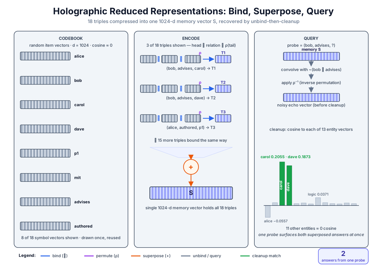The whole pipeline in one picture: random item vectors (left) are bound per triple and superposed into a single 1024-dimensional memory S (center); one unbind-then-cleanup probe for (bob, advises, ?) surfaces both stored advisees, carol at 0.2055 and dave at 0.1873 (right). Original diagram by the authors, created with AI assistance.

The commutativity ghost, and the permutation that exorcises it

A triple has three parts, so the obvious encoding binds all three: $(\mathbf{e}_h \circledast \mathbf{w}_r) \circledast \mathbf{e}_t$ for a triple with head $h$, relation $r$, and tail $t$. It is wrong, and the run demonstrates the failure before repairing it. Circular convolution is commutative and associative, so the triple product is a bag of factors: $(\mathbf{e}_{\text{alice}} \circledast \mathbf{w}_{\text{advises}}) \circledast \mathbf{e}_{\text{bob}}$ and $(\mathbf{e}_{\text{bob}} \circledast \mathbf{w}_{\text{advises}}) \circledast \mathbf{e}_{\text{alice}}$ are the same vector. Binding solved addition's bag-of-symbols problem at the fact level and then recreated it at the slot level.

Watch the failure mechanically. The naive memory stores $\sum (\mathbf{e}_h \circledast \mathbf{w}_r) \circledast \mathbf{e}_t$ over all 18 triples, among them (alice, advises, bob). Query it for bob's advisees by unbinding with the pair $\mathbf{e}_{\text{bob}} \circledast \mathbf{w}_{\text{advises}}$. The involution distributes over convolution (in the Fourier domain, the conjugate of a product is the product of the conjugates), so the probe is $\tilde{\mathbf{e}}_{\text{bob}} \circledast \tilde{\mathbf{w}}_{\text{advises}}$, and the stored alice-triple contributes the term

$$\mathbf{e}_{\text{alice}} \circledast \mathbf{w}_{\text{advises}} \circledast \mathbf{e}_{\text{bob}} \circledast \tilde{\mathbf{e}}_{\text{bob}} \circledast \tilde{\mathbf{w}}_{\text{advises}} \;=\; \mathbf{e}_{\text{alice}} \circledast \big(\mathbf{w}_{\text{advises}} \circledast \tilde{\mathbf{w}}_{\text{advises}}\big) \circledast \big(\mathbf{e}_{\text{bob}} \circledast \tilde{\mathbf{e}}_{\text{bob}}\big) \;\approx\; \mathbf{e}_{\text{alice}},$$

because each parenthesized factor is approximately the impulse $\boldsymbol{\delta}$. The probe cancels the factors bob and advises wherever they sat, and alice, bob's advisor, echoes back at exactly the strength a genuine advisee would. The run shows the ghost taking rank 1, ahead of both true answers:

why the tail slot needs ρ: query (bob, advises, ?) on the NAIVE
  memory Σ (e_h ⊛ w_r) ⊛ e_t  — ⊛ is commutative, so the stored
  triple (alice, advises, bob) echoes back alice at full strength:
  rank  entity  cosine
     1  alice    0.2271  * GHOST — bob's advisor, not his advisee
     2  dave     0.2083  * stored tail
     3  carol    0.1617  * stored tail

The standard repair is slot protection [1], in the form popularized by hyperdimensional computing as the permutation trick [3]: pass the tail through a fixed random permutation $\rho$ of the coordinates before binding, $\rho(\mathbf{x})[i] = \mathbf{x}[\text{perm}[i]]$ (vsa.py lines 128–133). A random permutation is not itself a convolution (a cyclic shift would be, which is why it must be random), so it does not commute with $\circledast$, and the encoding $(\mathbf{e}_h \circledast \mathbf{w}_r) \circledast \rho(\mathbf{e}_t)$ becomes directional: $\rho$ marks the tail slot the way a grammatical case ending marks the object of a sentence. Rerun the ghost calculation and it dissolves: the alice-triple now contributes $\mathbf{e}_{\text{alice}} \circledast \rho(\mathbf{e}_{\text{bob}}) \circledast \tilde{\mathbf{e}}_{\text{bob}}$ after cancellation, and $\rho(\mathbf{e}_{\text{bob}}) \circledast \tilde{\mathbf{e}}_{\text{bob}}$ has no impulse spike, because $\rho(\mathbf{e}_{\text{bob}})$ and $\mathbf{e}_{\text{bob}}$ are, statistically, unrelated random vectors. The ghost drops from cosine $0.2271$ to $-0.0557$ in the protected run below. Tail retrieval undoes the permutation after unbinding: the recovered tail estimate $\hat{\mathbf{t}}$ (on a whole boldface vector, the hat marks an estimate, not a Fourier coefficient) is $\hat{\mathbf{t}} = \rho^{-1}\big(\operatorname{unbind}(S,\, \mathbf{e}_h \circledast \mathbf{w}_r)\big)$.

The whole knowledge graph in one vector

Everything is now on the table. The memory is one line of algebra, a sum over the 18 triples of kg.py (the same 13-entity academic world every model in this volume trains on, kg.py lines 41–50), implemented verbatim in vsa.py lines 143–156:

def encode(triples: list[tuple[str, str, str]], cb: dict[str, np.ndarray],
           perm: np.ndarray | None = None) -> np.ndarray:
    """The holographic memory: every triple bound into one vector, all triples
    superposed by addition,

        S = Σ_{(h,r,t)} (e_h ⊛ w_r) ⊛ ρ(e_t).

    With ``perm=None`` the tail is left unprotected (ρ = identity) — the naive,
    order-blind encoding kept only to demonstrate its ghost answers."""
    S = np.zeros(next(iter(cb.values())).shape[0])
    for h, r, t in triples:
        tail = cb[t] if perm is None else permute(cb[t], perm)
        S += bind(bind(cb[h], cb[r]), tail)
    return S

Pause on what this line claims. Eighteen directional facts about specific individuals live in $1024$ floating-point numbers, roughly $57$ numbers per fact, with no index, no table, no training loop, and no gradient: encoding is one-shot algebra, the conceptual opposite of TransE's thousand epochs. Distributivity is what makes the memory queryable: unbinding the sum unbinds every term, so the probed triple yields its signal and the other 17 yield cross-talk noise. The query pipeline (vsa.py lines 159–170) is unbind, unpermute, clean up. Asked for bob's advisees, one probe of the protected memory returns:

query (bob, advises, ?) on the protected memory — one probe,
  then cleanup over the 13 entity vectors
  rank  entity  cosine
     1  carol    0.2055  * stored tail
     2  dave     0.1873  * stored tail
     3  logic    0.0371
  (alice now scores -0.0557 — the ghost is gone;
   both stored tails surface from a single unbinding: the
   superposition holds carol AND dave at once)

This table is the chapter's thesis in four rows. The knowledge graph stores two facts about bob's advising, (bob, advises, carol) and (bob, advises, dave), and both surface from a single unbinding, at cosines 0.2055 and 0.1873, with the best non-answer (the topic logic) far below at 0.0371 and the exorcised ghost alice at $-0.0557$. Superposition is not a compromise that stores one answer and loses the rest; the sum genuinely holds both bound pairs, and one probe reads both back, a claim the competency check at vsa.py lines 273–274 pins permanently. Note also why the winning cosines sit near 0.2 rather than the pair round trip's 0.66; the drop has two causes, and both are already derivable. First, the probe $\mathbf{e}_h \circledast \mathbf{w}_r$ is itself a two-factor binding, so the Fourier weight surviving on the tail is $W_j = \lvert \hat{e}_{h,j} \rvert^2 \lvert \hat{w}_{r,j} \rvert^2$, a product of two independent mean-1 exponentials; independence factors the second moment, $\mathbb{E}[W_j^2] = 2 \cdot 2 = 4$, and rerunning Step 3 of the fidelity derivation with $\sqrt{\mathbb{E}[W^2]} = 2$ gives a clean single-triple round trip of $1/\sqrt{4} = 1/2$, below the pair's $1/\sqrt{2}$ (the permutation $\rho$ changes nothing here, since permuting both vectors preserves norms and dot products). Second, the decoded vector's norm additionally carries the cross-talk of the other 17 superposed triples, so every cosine's denominator has grown again, pulling that clean $0.5$ down to the observed $0.2$. The signal has not shrunk; the deeper binding and the risen sea of cross-talk both live in the denominator. Run all 18 tail queries $(h, r, ?)$ against the stored tails and the little graph comes back whole:

  accuracy@1 = 18 / 18  (1.0000)

The capacity grid: where the calculus meets its wall

Eighteen triples in 1024 dimensions is a light load. The centerpiece experiment asks the only question that matters for scaling: how does recall behave as the load $k$ (the number of stored triples) grows and the dimension $d$ shrinks? The sweep (vsa.py lines 175–198) builds, for each cell, a fresh 50-entity, 5-relation vocabulary, stores $k$ uniformly random triples in one protected memory of dimension $d$, asks every stored triple back as a tail query, and scores accuracy at rank 1; a query counts as correct if the top-1 cleanup is any stored tail for its head-relation pair, since random triples can collide there, exactly like bob's two advisees. The committed grid:

accuracy@1	$k = 5$	$k = 18$	$k = 50$	$k = 200$
$d = 64$	0.6000	0.2778	0.1600	0.1250
$d = 256$	1.0000	0.6667	0.4800	0.1850
$d = 1024$	1.0000	1.0000	0.9200	0.6200

Read the two monotonicities first, because the competency checks pin one instance of each: accuracy at $(d = 1024, k = 18)$ must not fall below its value at $(d = 64, k = 18)$, nor below its value at $(d = 1024, k = 200)$ (vsa.py lines 276–279). Down any column, accuracy rises with dimension: at $k = 18$, from 0.2778 at $d = 64$ through 0.6667 at $d = 256$ to a perfect 1.0000 at $d = 1024$. Along any row, accuracy falls with load: at $d = 1024$, from 1.0000 at $k = 18$ down to 0.6200 at $k = 200$. Both slopes follow from one signal-to-noise argument, short enough to give in full. Probe a memory of $k$ triples for one of them. The probed triple contributes the signal, a vector whose cosine with the true tail is a fixed constant independent of $k$: the single-triple round-trip fidelity of approximately $1/2$ derived in the previous section, which sits below the pair fidelity $1/\sqrt{2}$ because the probe itself carries two bound factors. Each of the other $k - 1$ triples contributes a cross-talk vector: a convolution of items unrelated to the probe, hence a random-looking vector whose dot product with any fixed codebook item has mean zero and standard deviation of order $1/\sqrt{d}$. Independent noise terms add in variance, so the total cross-talk projected onto any candidate answer has standard deviation of order

$$\sigma_{\text{noise}} \;\sim\; \sqrt{\frac{k-1}{d}},$$

and the quantity that decides recall is the ratio of the fixed signal to that growing noise, the signal-to-noise ratio, which scales as $\sqrt{d/k}$. Every stored pair adds noise of order $1/\sqrt{d}$ to every other recall; dimension is the resource the noise is paid from. Recall at rank 1 additionally has to beat the maximum of the noise over the 50-item vocabulary, which is why accuracy erodes smoothly rather than cliff-diving: each added triple nudges the noise distribution upward, and one more query's margin drowns. The scaling even predicts the grid's diagonal: quadrupling both $d$ and $k$ should roughly preserve the ratio, and the two cells land in the same regime, 0.4800 at $d = 256, k = 50$ against 0.6200 at $d = 1024, k = 200$; the second number runs somewhat high because at $k = 200$ over a 50-entity vocabulary many head-relation pairs hold several stored tails, and the any-stored-tail scoring is more lenient there. HRR's original capacity analysis makes this argument exact, deriving the dimension needed to store $k$ pairs at a target error probability; the scaling law is the same [1].

Graceful degradation: the feature that is also the price

Look at what the grid does not contain: a crash. At $d = 64$ with $k = 200$ triples crammed into a 64-dimensional vector, the memory still answers every query; it is merely wrong 87.5 percent of the time. Nothing raised an exception, nothing refused, nothing reported "memory full." This is graceful degradation, and the hyperdimensional-computing literature is right to celebrate it [3]. Contrast Volume 2's completion engine: overload it with a contradiction and it derives ⊥ (the contradiction symbol, Volume 2's unsatisfiable bottom concept), names the concept at fault, and shows the axioms responsible. The symbolic system is brittle and loud about it; the holographic memory is robust and silent. Damage half the coordinates of $S$ and recall degrades in proportion; damage half the entries of a symbol table and the system halts. For hardware, for noisy sensors, for biology, the VSA behavior is the desirable one.

The price is the silence. A cleanup cosine of 0.2055 comes with no certificate: when the memory returns a wrong tail at $d = 64$, the wrong answer arrives through the same interface, a name and a score, as every right one. There is no ⊥, no proof trace, no way to ask the vector why. The failures are statistically predictable in aggregate (that is what the grid is) and individually invisible. This trade, robustness purchased with auditability, is the recurring bargain of every neural representation in this volume, isolated here in its purest form, and it is the charge sheet the volume's closing verdict chapter will weigh.

The family in one table

Circular convolution is one choice of binding operator among several that satisfy the requirements list; the family that results is what the umbrella term Vector Symbolic Architectures names [4]. The members differ in their vector space and binding algebra but share the architecture: random item vectors, a dissimilarity-preserving binding, additive superposition, approximate unbinding, cleanup.

architecture	vector space	binding	unbinding	the trade
Tensor product [2]	$\mathbb{R}^{d \times d}$, growing per level	outer product $\mathbf{a}\mathbf{b}^{\top}$	inner-product contraction, exact	exact recovery, but dimension squares with every nesting level
HRR [1]	$\mathbb{R}^{d}$, $\mathcal{N}(0, 1/d)$ items	circular convolution $\circledast$, $O(d \log d)$ via FFT	involution $\tilde{\mathbf{a}}$, approximate ($\cos \approx 1/\sqrt{2}$)	fixed dimension at any depth, paid for with intrinsic noise and cleanup
Binary spatter codes [3]	dense binary $\lbrace 0,1 \rbrace^{d}$	coordinatewise XOR	XOR again, self-inverse and exact	binding exact and cheap; superposition (majority vote) is where the noise lives
MAP (Multiply-Add-Permute) [4]	bipolar $\lbrace -1,+1 \rbrace^{d}$	coordinatewise multiplication	multiplication again, self-inverse	on strictly bipolar vectors binding is XOR in disguise (equally dissimilarity-preserving); the appeal is the trivial hardware mapping, and exactness lasts only while vectors stay bipolar: once superposed, integer-valued vectors unbind only approximately

The tensor product row is the origin story: binding as the outer product came first, as the connectionist answer to variable binding [2], and every later row is a lossy compression of it back into fixed dimension, choosing where to spend the information loss. One sentence of foreshadowing is owed here: the same superposition calculus, many more features than dimensions coexisting as nearly orthogonal directions in one activation vector, is now the working hypothesis for how trained transformers pack their internal features, which makes this chapter's noise arithmetic unexpectedly relevant to interpreting the models of the previous chapter [5].

The unsolved part

The cleanup memory can only return symbols it was given. Every recovery in this chapter ended in a nearest-neighbor sweep over a fixed codebook of stored items, and the codebook's vectors are random: $\mathbf{w}_{\text{advises}}$ carries no more relation to a hypothetical $\mathbf{w}_{\text{supervises}}$ than to $\mathbf{e}_{\text{p2}}$, because near-orthogonality of everything is precisely the design. That design is what makes recall clean, and it is also a wall. Reasoning, as Volumes 1 and 2 practiced it, constantly needs to match symbols that are merely similar: to notice that a rule about advising should probably fire for a fact about supervising. A VSA memory queried with $\mathbf{w}_{\text{supervises}}$ returns noise, exactly as designed. One can inject similarity by constructing item vectors that share components, and HRR anticipated this, but then the noise analysis, which assumed independence everywhere, must be redone with every shared component acting as systematic cross-talk, and nobody has a general account of how much structured similarity a superposed memory can carry before its capacity argument collapses. How to keep this algebra of exact structure while admitting graded similarity between symbols, and then to chain such graded matches through multi-step rules with a meaningful composite score, is genuinely open, and it is the precise doorway to the next chapter.

Why it matters

For the neuro-symbolic program, this chapter is an existence proof with teeth. A recurring skeptical position holds that vectors can encode associations but not structure, that "who did what to whom" inherently needs pointers and symbol tables. The committed run refutes the strong version of that claim with 1024 floats: a full directional knowledge graph, stored in one vector by pure algebra, queried by pure algebra, 18 for 18, with the failure mode not hidden but measured on a grid. Equally important is how: with no training. Binding, superposition, and unbinding are fixed differentiable operations (the FFT is linear and the pointwise product bilinear, so bind, superpose, and unbind compose into a smooth map); the one non-differentiable step is the cleanup's argmax over the codebook (argmax is the pick-the-largest operation: it returns the symbol with the highest cosine), and when gradients must flow it is replaced by a softmax over the codebook cosines, which is attention over the vocabulary, the previous chapter's operator returning in a new role. With that substitution the whole pipeline can sit inside a learned model and pass gradients, which is exactly the role structured vector operations play in Volume 4's differentiable-logic systems. And the capacity grid's lesson, that structure held in superposition is real but budgeted, with dimension the currency and cross-talk the tax, is the quantitative frame to carry into every architecture that claims to represent relations in activation space, transformers included. Attention gave a differentiable where to look; this chapter gave a differentiable what goes with what; the remaining gap, a differentiable matches whom, is one chapter away.

Key terms

• Vector Symbolic Architecture (VSA): a family of representation schemes over high-dimensional random vectors, built from a binding operation, additive superposition, approximate unbinding, and a cleanup memory.
• Binding ($\circledast$): the composition of two vectors into one of the same dimension, near-orthogonal to both inputs; in HRR, circular convolution $(\mathbf{a} \circledast \mathbf{b})[i] = \sum_k a[k]\,b[(i-k) \bmod d]$.
• Superposition: plain vector addition as storage; many bound pairs coexist in one vector, each recoverable, each adding cross-talk noise to the others.
• Holographic Reduced Representation (HRR): the real-valued VSA using circular convolution, computable in $O(d \log d)$ by the FFT through the convolution theorem.
• Involution ($\tilde{\mathbf{a}}$): index reversal modulo $d$, HRR's stable approximate inverse; $\mathbf{a} \circledast \tilde{\mathbf{a}}$ approximates the impulse $\boldsymbol{\delta}$ scaled by $\lVert \mathbf{a} \rVert^2$, giving round-trip fidelity near $1/\sqrt{2}$.
• Cleanup memory: the nearest-neighbor sweep (by cosine) over the item codebook that converts a noisy decoded vector back into an exact stored symbol.
• Slot protection (permutation trick): a fixed random coordinate permutation $\rho$ applied to one argument before binding; because $\rho$ does not commute with convolution, it makes the encoding directional and kills commutativity ghosts.
• Capacity / graceful degradation: recall accuracy governed by a signal-to-noise ratio scaling as $\sqrt{d/k}$ for $k$ items stored in $d$ dimensions; overload degrades accuracy smoothly and silently rather than failing loudly.

Where this leads

Vector Symbolic Architectures match stored symbols exactly, by construction, and match everything else not at all; the codebook knows identity but not kinship. The next chapter, Soft Unification, takes the step this algebra cannot: it replaces the equality test at the heart of symbolic proof with a kernel on embedding vectors, so that advises and a near-synonym can match at 0.98 instead of 0, and it threads such graded matches through entire proof chains, scoring a derivation by its weakest link. Where this chapter kept symbols exact and made structure vectorial, the next makes the symbols themselves negotiable, and inherits a new obligation: deciding how good a match is good enough.

---

Companion code: examples/neural/vsa.py implements the full pipeline, both binding implementations and their agreement check, the fidelity round trip, the naive-encoding ghost, the protected 18-triple memory with all tail queries, and the capacity sweep, all driven by one seeded generator over the knowledge graph fixed in examples/neural/kg.py. Run python3 vsa.py from examples/neural/ to reproduce every number in this chapter; the acceptance harness examples/neural/validate.py re-executes its competency asserts (the 1e-10 FFT gate, the fidelity band, the unrelated-vector orthogonality check, the naive ghost's appearance, the carol-and-dave top-2, the 16-of-18 floor, and the two capacity-monotonicity spot checks) as part of the volume's verdict.