Relational GNNs: R-GCN and Beyond

📍 Where we are: Part IV · Graph Neural Networks and Their Ceiling — Chapter 13. Message Passing built the two-layer Graph Convolutional Network (GCN) blueprint but got there by flattening our knowledge graph into an undirected, unlabeled ball of edges; this chapter puts the five relations back into the message.

The previous chapter made a quiet sacrifice. To run the GCN blueprint, gnn.py collapsed all 18 triples of the academic world into one symmetric adjacency matrix: advises(bob, dave) and about(p1, logic) became indistinguishable 1-entries. The model still classified three of the four held-out nodes correctly, but it did so with one hand tied behind its back, because in a knowledge graph the type of an edge is most of what the edge says. An incoming authored edge means "you are a paper"; an incoming advises edge is strong evidence you are a student (three of the four advisees here are); an untyped model hears only "you have a neighbor." This chapter restores the types. The Relational Graph Convolutional Network (R-GCN) gives every relation its own weight matrix, learns them all jointly by the same manual backpropagation as before, and then confronts the bill: parameters that grow linearly with the number of relations, and the basis decomposition that caps them [1]. Every number below comes from the committed run of examples/neural/rgcn.py.

The simple version

Imagine a company mailroom that receives letters in five languages. The cheap setup hires one translator who renders everything into a single bland paraphrase: a legal notice from Berlin and a love letter from Lisbon come out sounding the same, and the meaning that lived in which language it arrived in is gone. The R-GCN setup hires one dedicated translator per language, plus one per language for outgoing mail, plus a clerk who files your own notes back to you: eleven specialists in total. Translations get faithful, but the payroll now grows with every language you add. The final trick is to hire just two brilliant polyglots and describe each language's translator as a personal blend of the two ("70 percent of polyglot one, 30 percent of polyglot two"). That blend is the basis decomposition: almost all the skill is shared, and each language costs only two mixing numbers.

What this chapter covers

• Why collapsing edge types is lossy: argued on our graph, where four nodes of four different classes share the same degree, fourteen of eighteen edges join nodes of different classes, and only the relation labels can tell an institution from a professor.
• The R-GCN propagation rule, symbol by symbol: per-relation neighborhoods $N_r(i)$, the per-relation normalizer $c_{i,r}$, the separate self-loop matrix $W_0$, and why inverse relations must be added before information can flow both ways along a directed edge.
• The parameter ledger, computed not asserted: 880 weights per layer times two layers for the full model, quoted from arrays, and why linear-in-$\lvert\mathcal{R}\rvert$ growth is unaffordable on real knowledge graphs.
• Basis decomposition, derived: $W_r = \sum_b a_{rb} V_b$ with $B = 2$ shared prototypes, the gradient through the mixture worked out entry by entry (a weighted sum for $V_b$, a trace for $a_{rb}$), and the committed count of 364 parameters beside the full model's 1760.
• The three-way ablation as the empirical spine: untyped, full, and basis models trained by the identical code, seed, and task, with held-out accuracy 1/4, 4/4, and 3/4, read honestly.
• Regularization as the real-world lesson: why the basis is not merely a compression trick but the anti-overfitting device for the rare relations that dominate knowledge graphs at scale.
• Beyond R-GCN: CompGCN's composition of relation and entity embeddings inside the message, NBFNet's path-based Bellman–Ford view of link prediction, and the relation-agnostic direction they opened.

Why one weight matrix is not enough

Start from what the previous chapter's model actually computes. In an untyped GCN, the message node $i$ receives from a neighbor $j$ is $W \mathbf{h}_j$: the neighbor's current feature vector $\mathbf{h}_j$, pushed through the single shared weight matrix $W$ of that layer. The matrix does not know, and cannot be told, which relation delivered the message. On our graph that is a real loss, because the five relations implement five incompatible transformations:

relation	connects	edges	example triple
advises	person → person	4	(alice, advises, bob)
affiliated	person → institution	5	(carol, affiliated, cmu)
authored	person → paper	4	(bob, authored, p1)
cites	paper → paper	2	(p2, cites, p1)
about	paper → topic	3	(p1, about, logic)

An advises edge maps evidence about a person into evidence about another person; an about edge maps evidence about a paper into evidence about a topic. Forcing one $W$ to serve both means $W$ must be a compromise, an average of transformations that should point in different directions. The failure mode has a name: heterophily, the situation in which connected nodes tend to carry different labels, so that naively averaging neighbors pulls a node's representation toward the wrong class [2]. Citation networks, where linked papers usually share a topic, are homophilous and forgiving; knowledge graphs are heterophilous by construction. Count it on ours: of the 18 edges, only four join nodes of the same class (alice→bob among professors, carol→erin among students, and the two cites edges among papers). The other fourteen cross class boundaries, and for those fourteen the relation label is the signal.

The task from the previous chapter makes the loss concrete. We are doing 5-class entity typing with identity-free features: each node's input is a one-hot encoding of its degree, so everything the model learns must come from structure (rgcn.py lines 67–85). Now look at the degree-3 nodes: alice is a Professor, cmu an Institution, dave a Student, and p3 a Paper. Four nodes, four classes, identical input features. The only thing that can separate them is their neighborhoods, and their neighborhoods differ mostly in type: all three of cmu's edges are incoming affiliated, dave's one incoming edge is advises, p3's is authored. An untyped model must hope the mixture of degrees in each neighborhood happens to differ; a typed model can simply read which channel the messages arrive on. The ablation at the end of this chapter measures exactly this gap.

The propagation rule, symbol by symbol

The R-GCN layer update for node $i$ is [1]:

$$\mathbf{h}_i' \;=\; \mathrm{ReLU}\!\left( \sum_{r \in \mathcal{R}} \; \sum_{j \in N_r(i)} \frac{1}{c_{i,r}}\, W_r\, \mathbf{h}_j \;+\; W_0\, \mathbf{h}_i \right).$$

Decode it one symbol at a time, plain language first. The index $i$ ranges over the $N = 13$ nodes, and $\mathbf{h}_i$ is node $i$'s current feature vector (at the input layer, its one-hot degree, a vector of length $d_{\text{in}} = 5$). The set $\mathcal{R}$ collects the relation types. For each relation $r$, the per-relation neighborhood $N_r(i) = \lbrace j : (j, r, i) \in E \rbrace$ is the set of nodes $j$ that have an $r$-edge into $i$, where $E$ is the edge set, the 18 directed typed triples of our graph; the sum over $j \in N_r(i)$ gathers one message per such neighbor. Each relation gets its own weight matrix $W_r$, so the message $W_r \mathbf{h}_j$ is transformed differently depending on which relation carried it: that is the entire repair. The normalizer $c_{i,r} = \lvert N_r(i)\rvert$ is the per-relation in-degree, the count of $r$-neighbors of $i$; dividing by it turns each relation's message pile into an average, so a node with five affiliated neighbors is not simply louder than a node with one. Finally $W_0$ is a separate self-loop matrix: node $i$'s own vector is passed through its own transformation and added, so a node never loses itself in its neighbors' voices. ReLU (Rectified Linear Unit), the elementwise map $\max(0, \cdot)$, is the same nonlinearity as before.

One subtlety in $N_r(i)$ deserves a careful walk, because getting it wrong silences half the graph. The definition reads messages along edge direction: for the triple (alice, advises, bob), alice $\in N_{\text{advises}}(\text{bob})$, so the edge delivers a message to bob, its tail; alice, the head, receives nothing from it. On our graph that is fatal: alice appears as the tail of no triple (all three of her edges point outward), so under the base relations alone her update would be $\mathrm{ReLU}(W_0 \mathbf{h}_{\text{alice}})$, a function of her own degree and nothing else. The standard fix is to add, for every relation $r$, an inverse relation $r^{-1}$ whose edges run the other way: (alice, advises, bob) also creates bob $\in N_{\text{advises}^{-1}}(\text{alice})$, with its own weight matrix $W_{r^{-1}}$ [1]. Now alice hears from bob through the advises⁻¹ channel, and hears it typed: being the adviser and being the advisee arrive on different channels with different matrices, exactly the distinction "Professor versus Student" needs.

The companion code builds all of this as a stack of adjacency matrices, one per channel: 5 base relations, 5 inverses, and the self-loop as its own channel with $\hat{A}_{\text{self}} = I$, the identity matrix (ones on the diagonal, zeros elsewhere, so this channel hands each node its own vector), for 11 channels total (rgcn.py lines 91–133):

    channels: list[tuple[str, np.ndarray]] = []
    if typed:
        for rel in RELATIONS:                     # base: message head → tail
            A = np.zeros((N, N))
            for h, r, t in TRIPLES:
                if r == rel:
                    A[E_ID[t], E_ID[h]] = 1.0
            channels.append((rel, A))
        for rel in RELATIONS:                     # inverse: message tail → head
            A = np.zeros((N, N))
            for h, r, t in TRIPLES:
                if r == rel:
                    A[E_ID[h], E_ID[t]] = 1.0
            channels.append((rel + "⁻¹", A))
    else:
        A = np.zeros((N, N))                      # one untyped, symmetric channel
        for h, _, t in TRIPLES:
            A[E_ID[t], E_ID[h]] = 1.0
            A[E_ID[h], E_ID[t]] = 1.0
        channels.append(("edge", A))
    channels.append(("self", np.eye(N)))          # the self-loop channel

    names = [name for name, _ in channels]
    A_hat = np.stack([A for _, A in channels])
    # Row normalization: divide row i of Â_r by c_{i,r} = |N_r(i)|.
    c = A_hat.sum(axis=2, keepdims=True)
    A_hat = A_hat / np.where(c == 0.0, 1.0, c)

Note the else branch: the same function, asked for typed=False, builds the untyped setting (every edge in both directions collapsed into one relation, plus the self-loop, 2 channels). That branch is the ablation we will train later, living inside the identical code path so that nothing but the typing differs. The row normalization at the bottom implements $1/c_{i,r}$: entry $(i, j)$ of $\hat{A}_r$ becomes $1/c_{i,r}$ if $j \in N_r(i)$ and 0 otherwise, with all-zero rows left alone. Running the module prints the channels and grounds the normalizer in one concrete row; this is real committed output:

11 relation channels (5 base + 5 inverse + 1 self-loop), edges per channel:
  about:3  advises:4  affiliated:5  authored:4  cites:2  about⁻¹:3  advises⁻¹:4  affiliated⁻¹:5  authored⁻¹:4  cites⁻¹:2  self:13
  e.g. c_(cmu,affiliated) = 3 (carol, dave, erin): each neighbour contributes weight 1/3 = 0.3333

Because every $\hat{A}_r$ already carries its normalizer and the self-loop channel contributes the $W_0 \mathbf{h}_i$ term, the whole layer collapses into one matrix equation over the feature matrix $H$ (one row per node):

$$H' \;=\; \mathrm{ReLU}\!\left( \sum_{r=1}^{R} \hat{A}_r\, H\, W_r \right), \qquad R = 11,$$

where the code follows the row-vector convention, so each $W_r$ multiplies on the right (rgcn.py lines 195–218). At the output layer the ReLU is replaced by the softmax classifier head, exactly as in the previous chapter (lines 209–217). This is the form the forward and backward passes below manipulate.

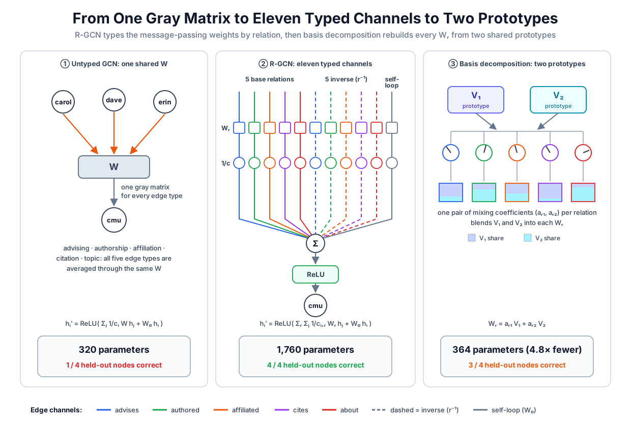From one gray matrix to eleven typed channels to two shared prototypes: the R-GCN propagation rule and its parameter bill on the academic graph. Original diagram by the authors, created with AI assistance.

The parameter ledger, computed not asserted

Typed weights cost weights. A layer that maps $d_{\text{in}}$ input features to $d_{\text{out}}$ outputs needs one $d_{\text{in}} \times d_{\text{out}}$ matrix per channel, so the per-layer count is $R \cdot d_{\text{in}} \cdot d_{\text{out}}$. Our network has two layers with hidden width 16 (rgcn.py lines 42–46): layer 1 maps the 5 degree features to 16 hidden units, layer 2 maps 16 hidden units to the $K = 5$ classes. The module counts the parameters from the actual arrays rather than from a formula (param_counts, lines 182–190), and prints:

parameters (counted from the actual arrays)
  layer     full (11 relations)      basis (B=2)
  layer 1   11×(5×16) =   880        2×(5×16) + 11×2 =  182
  layer 2   11×(16×5) =   880        2×(16×5) + 11×2 =  182
  total                 1760                          364   (4.8× fewer)

Check the arithmetic once: $11 \times 5 \times 16 = 880$ for layer 1, the same product reversed for layer 2, and $880 + 880 = 1760$ trainable weights. The untyped ablation, with only 2 channels, needs $2 \times 80 = 160$ per layer, 320 in total. The point of the ledger is the scaling law it exposes: the count is linear in the number of relations, and every relation multiplies the full $d_{\text{in}} \cdot d_{\text{out}}$ block. Our toy pays a factor of 5.5 over the untyped model for its 5 relations. A real benchmark graph makes the growth concrete: FB15k-237, the standard Freebase-derived benchmark whose relation vocabulary is exactly 237, would need $2 \times 237 + 1 = 475$ channels; at a hidden width of 500, a single hidden-to-hidden layer under our formula would hold $475 \times 500 \times 500 \approx 1.19 \times 10^8$ weights. Knowledge graphs with thousands of relation types exist, and for them the full parameterization is simply not writable down, let alone trainable on the handful of edges most relations have [1].

Basis decomposition: eleven matrices from two

The repair is to stop giving each relation a free matrix and instead give each relation a recipe. Fix a small number $B$ of shared basis matrices $V_1, \ldots, V_B$ (here $B = 2$), each of the full $d_{\text{in}} \times d_{\text{out}}$ size, and write every relation's matrix as a learned linear mixture of them [1]:

$$W_r \;=\; \sum_{b=1}^{B} a_{rb}\, V_b .$$

The scalars $a_{rb}$ are the mixing coefficients: relation $r$'s personal blend of the $B$ shared prototypes, $B$ numbers per relation. The parameter count per layer becomes $B \cdot d_{\text{in}} \cdot d_{\text{out}} + R \cdot B$: for layer 1, $2 \times 80 + 11 \times 2 = 182$, and 364 in total, the number quoted in the ledger above, 4.8 times fewer than the full model. Read the formula structurally: the expensive $d_{\text{in}} \cdot d_{\text{out}}$ block is now multiplied by the constant $B$, not by $R$, and the only term that grows with the relation vocabulary is the cheap $R \cdot B$ table of coefficients. Adding a relation costs two numbers instead of eighty. The forward pass materializes each $W_r$ from the recipe before propagating (rgcn.py lines 169–179):

    if params["kind"] == "full":
        return params["W1"], params["W2"]
    R = params["a1"].shape[0]
    W1 = np.zeros((R, D_IN, HIDDEN))
    W2 = np.zeros((R, HIDDEN, K))
    for r in range(R):
        for b in range(BASES):
            # W_r = Σ_b a_{rb} V_b   (same B bases shared by all R relations)
            W1[r] += params["a1"][r, b] * params["V1"][b]
            W2[r] += params["a2"][r, b] * params["V2"][b]
    return W1, W2

Training the typed network: every gradient by hand

Both parameterizations train on the same task as the previous chapter: masked cross-entropy over the 9 labeled nodes, with bob, dave, p2, and cmu held out, full-batch gradient descent at learning rate $\eta = 0.5$ for 400 epochs from seed 0 (train_model, rgcn.py lines 223–310). The loss is

$$L \;=\; -\frac{1}{\lvert T\rvert} \sum_{i \in T} \ln p_{i,\,y_i}, \qquad \lvert T\rvert = 9,$$

where $T$ is the set of labeled training nodes, $y_i$ is node $i$'s true class, $\ln$ is the natural logarithm (the logarithm base $e$), and $p_{i,k}$ is the softmax probability the network assigns to class $k$ for node $i$. The gradient at the logits is the same softmax-plus-cross-entropy residual that drove Message Passing, and it is short enough to rederive in place, so this chapter stands on its own. Write $z_{i,k}$ for node $i$'s logit for class $k$ (the pre-softmax score) and $c$ for the true class, so that $p_{i,k} = e^{z_{i,k}} / \sum_{k'} e^{z_{i,k'}}$, where the summation index $k'$ runs over the 5 classes. The logarithm turns that quotient into a difference, giving one node's loss as

$$L_i \;=\; -\ln p_{i,c} \;=\; -z_{i,c} + \ln \sum_{k'} e^{z_{i,k'}} .$$

Differentiate each term with respect to one logit $z_{i,k}$. The first term is linear: $\partial(-z_{i,c})/\partial z_{i,k}$ is $-1$ when $k = c$ and $0$ otherwise, which is exactly $-y_{i,k}$ for the one-hot target $y_{i,k}$. The second term goes through the chain rule. Abbreviate the normalizing sum as $S = \sum_{k'} e^{z_{i,k'}}$; then $\partial(\ln S)/\partial z_{i,k} = (1/S)\,\partial S/\partial z_{i,k}$, and because only the $k' = k$ summand of $S$ contains $z_{i,k}$, its derivative is $\partial S/\partial z_{i,k} = e^{z_{i,k}}$. The resulting quotient $e^{z_{i,k}}/S$ is the softmax probability $p_{i,k}$ itself. Adding the two pieces:

$$\frac{\partial L_i}{\partial z_{i,k}} \;=\; p_{i,k} - y_{i,k} .$$

Averaged over the 9 labeled rows and zeroed elsewhere by the mask, this is G2 = (P - Y) * mask / n_tr (rgcn.py line 254).

What is new is the gradient's route through the typed channels. Write $G$ for $\partial L/\partial Z_2$ (a $13 \times 5$ matrix, one row per node, one column per class) and $M_r = \hat{A}_r H_1$ for relation $r$'s aggregated, normalized neighborhood features, so that layer 2 reads $Z_2 = \sum_r M_r W_{2,r}$. To differentiate with respect to one relation's matrix $W_{2,\rho}$ (the index $\rho$ picks out one channel; $m$ indexes the 16 hidden coordinates, $k$ and $n$ index the 5 classes), expand entrywise:

$$(Z_2)_{ik} \;=\; \sum_{r=1}^{R} \sum_{m=1}^{16} (M_r)_{im}\, (W_{2,r})_{mk} \quad\Longrightarrow\quad \frac{\partial (Z_2)_{ik}}{\partial (W_{2,\rho})_{mn}} \;=\; (M_\rho)_{im}\,\delta_{kn},$$

where $\delta_{kn}$ is the Kronecker delta, equal to 1 when $k = n$ and 0 otherwise: entry $(m, n)$ of channel $\rho$'s matrix touches only column $n$ of the logits, and only through channel $\rho$. The chain rule then sums the products of the two:

$$\frac{\partial L}{\partial (W_{2,\rho})_{mn}} \;=\; \sum_{i,k} G_{ik}\, (M_\rho)_{im}\,\delta_{kn} \;=\; \sum_{i} (M_\rho^{\top})_{mi}\, G_{in} \;=\; \big( (\hat{A}_\rho H_1)^{\top} G \big)_{mn}.$$

Each channel gets its own gradient, built from its own aggregated features. The hidden state collects contributions from all channels; expanding $(Z_2)_{ik} = \sum_r \sum_j \sum_m (\hat{A}_r)_{ij} (H_1)_{jm} (W_{2,r})_{mk}$ and differentiating with respect to $(H_1)_{jm}$ gives $\sum_r (\hat{A}_r)_{ij}(W_{2,r})_{mk}$. The chain rule then contracts this against $G$ over every logit entry, and rewriting each factor through its transpose exposes the matrix product:

$$\frac{\partial L}{\partial (H_1)_{jm}} \;=\; \sum_{i,k} G_{ik} \sum_{r=1}^{R} (\hat{A}_r)_{ij}\, (W_{2,r})_{mk} \;=\; \sum_{r=1}^{R} \sum_{i,k} (\hat{A}_r^{\top})_{ji}\, G_{ik}\, (W_{2,r}^{\top})_{km} \;=\; \sum_{r=1}^{R} \big( \hat{A}_r^{\top}\, G\, W_{2,r}^{\top} \big)_{jm},$$

an identity at every entry $(j, m)$ at once, so as matrices

$$\frac{\partial L}{\partial H_1} \;=\; \sum_{r=1}^{R} \hat{A}_r^{\top}\, G\, W_{2,r}^{\top}.$$

The transpose on $\hat{A}_r$ matters here in a way it did not in the previous chapter: the GCN's operator was symmetric, but $\hat{A}_r$ is directional, and $\hat{A}_r^{\top}$ runs every arrow backward, sending the credit for node $i$'s error to the neighbors $j$ that spoke to it. The ReLU gate and the layer-1 weight gradients then repeat the pattern. All of it is implemented verbatim (rgcn.py lines 251–269):

        # ---- Backward pass (all gradients hand-derived) -----------------
        # Softmax + cross-entropy cancel to the classic residual:
        #   ∂L/∂Z2[i,:] = (p_i − y_i)/|T| for labelled i, 0 for held-out i.
        G2 = (P - Y) * mask / n_tr
        # Layer-2 weights and hidden state.  From Z2 = Σ_r (Â_r H1) W2_r:
        #   ∂L/∂W2_r = (Â_r H1)ᵀ G2          (each channel's own gradient)
        #   ∂L/∂H1   = Σ_r Â_rᵀ (G2 W2_rᵀ)   (the message, transposed back)
        dW2 = np.zeros_like(W2)
        dH1 = np.zeros_like(H1)
        for r in range(R):
            dW2[r] = (A_hat[r] @ H1).T @ G2
            dH1 += A_hat[r].T @ (G2 @ W2[r].T)
        # ReLU: H1 = max(0, Z1)  ⟹  ∂L/∂Z1 = ∂L/∂H1 ⊙ 1[Z1 > 0]
        G1 = dH1 * (Z1 > 0.0)
        # Layer-1 weights.  From Z1 = Σ_r (Â_r X) W1_r:
        #   ∂L/∂W1_r = (Â_r X)ᵀ G1
        dW1 = np.zeros_like(W1)
        for r in range(R):
            dW1[r] = (A_hat[r] @ X).T @ G1

For the full model, the update is the plain descent step $\theta \leftarrow \theta - \eta\, \partial L/\partial \theta$ on each $W_r$ stack. The basis model needs one more application of the chain rule, because the trainable objects are the prototypes $V_b$ and the coefficients $a_{rb}$, and $L$ reaches them only through the materialized $W_r = \sum_b a_{rb} V_b$. Take the two derivatives entry by entry, writing $\beta$ for the one fixed prototype being differentiated with respect to, kept distinct from the running summation index $b$, and $(m', n')$ for one fixed entry of that prototype. Since $(W_r)_{mn} = \sum_b a_{rb} (V_b)_{mn}$, the derivative of $(W_r)_{mn}$ with respect to entry $(m', n')$ of prototype $V_\beta$ is $a_{r\beta}\,\delta_{mm'}\,\delta_{nn'}$: the coefficient when the entries line up, zero otherwise. Summing the chain rule over every relation and every entry, the deltas collapse the inner sum:

$$\frac{\partial L}{\partial (V_\beta)_{m'n'}} \;=\; \sum_{r=1}^{R} \sum_{m,n} \frac{\partial L}{\partial (W_r)_{mn}}\, a_{r\beta}\,\delta_{mm'}\,\delta_{nn'} \;=\; \sum_{r=1}^{R} a_{r\beta}\, \frac{\partial L}{\partial (W_r)_{m'n'}},$$

which holds at every entry at once, so as matrices $\partial L/\partial V_\beta = \sum_r a_{r\beta}\, \partial L/\partial W_r$. Prototype $\beta$ sits inside every relation's matrix, so its gradient is the coefficient-weighted sum of all eleven per-relation gradients. For one coefficient $a_{\rho\beta}$, the derivative of $(W_\rho)_{mn}$ is simply $(V_\beta)_{mn}$, so

$$\frac{\partial L}{\partial a_{\rho\beta}} \;=\; \sum_{m,n} \frac{\partial L}{\partial (W_\rho)_{mn}}\, (V_\beta)_{mn} \;=\; \Big\langle V_\beta,\ \frac{\partial L}{\partial W_\rho} \Big\rangle_F \;=\; \operatorname{tr}\!\Big( V_\beta^{\top}\, \frac{\partial L}{\partial W_\rho} \Big),$$

the Frobenius inner product of the prototype with that relation's gradient (the sum of the products of matching entries, equal to the trace $\operatorname{tr}$, the sum of diagonal entries, of $V_\beta^{\top} \partial L/\partial W_\rho$). It measures how much sliding relation $\rho$'s blend toward prototype $\beta$ would reduce the loss. Both formulas appear as written (rgcn.py lines 276–288):

            # Chain rule through the decomposition W_r = Σ_b a_{rb} V_b:
            #   ∂L/∂V_b   = Σ_r a_{rb} · ∂L/∂W_r      (V_b sits inside every W_r)
            #   ∂L/∂a_{rb} = ⟨V_b, ∂L/∂W_r⟩_F         (Frobenius inner product)
            for a_key, v_key, dW in (("a1", "V1", dW1), ("a2", "V2", dW2)):
                a, V = params[a_key], params[v_key]
                dV = np.zeros_like(V)
                da = np.zeros_like(a)
                for r in range(R):
                    for b in range(BASES):
                        dV[b] += a[r, b] * dW[r]
                        da[r, b] = float(np.sum(V[b] * dW[r]))
                a -= LR * da
                V -= LR * dV

All three models descend to essentially zero training loss; the committed loss trace shows the typed models getting there far faster (the untyped model's first-epoch loss sits near the uniform-guess value $\ln 5 \approx 1.6094$, while the full model starts higher because eleven summed channels give its initial logits a larger spread):

epoch	untyped	R-GCN full	R-GCN basis
1	1.6267	2.0372	1.6622
10	0.8565	0.0857	0.2525
50	0.1172	0.0072	0.0028
100	0.0369	0.0030	0.0009
200	0.0127	0.0013	0.0004
400	0.0048	0.0006	0.0002

The ablation: what typed weights bought

Training loss is not the question; all three models fit their 9 labels perfectly. The question is the four nodes no model ever saw a label for, and here is the committed answer, node by node and then summarized (run, rgcn.py lines 315–345, trains all three exhibits):

held-out predictions (4 nodes never seen with a label)
  node   true          untyped          R-GCN full       R-GCN basis
  bob    Professor     Student      ✗   Professor    ✓   Professor    ✓
  dave   Student       Paper        ✗   Student      ✓   Student      ✓
  p2     Paper         Paper        ✓   Paper        ✓   Paper        ✓
  cmu    Institution   Professor    ✗   Institution  ✓   Professor    ✗

relation ablation — same code, same seed, only the typing differs
  model                        params   train acc     held-out acc
  untyped (1 edge relation)       320   9/9 1.0000    1/4 0.2500
  R-GCN full (11 relations)      1760   9/9 1.0000    4/4 1.0000
  R-GCN basis (B=2)               364   9/9 1.0000    3/4 0.7500

Read the mechanism off the rows. The untyped model gets only p2 right, exactly the failure the degree-collision argument predicted: stripped of relation labels, bob's mixed neighborhood of a professor, two students, a paper, and an institution reads as "student," and cmu, whose entire identity is being the target of three affiliated edges, reads as "professor." The full R-GCN gets all four, because the channels carry the type information directly: cmu's messages all arrive on affiliated; dave's only incoming edge arrives on advises, the channel whose incoming side the training labels associate with Student (carol and erin, the two labeled advisees, are both Students); and bob is the only held-out node that sends on advises twice, which the advises⁻¹ channel delivers back to him. The basis model keeps bob, dave, and p2 but loses cmu to "professor": with two shared prototypes serving eleven channels, affiliated cannot maintain a fully distinct transformation, and cmu is precisely the node whose evidence lives in that one channel.

Two honesty notes before generalizing. First, the untyped row is not the previous chapter's GCN rerun: gnn.py used the symmetric operator $D^{-1/2}(A+I)D^{-1/2}$ (the previous chapter's normalization, where $A$ is the untyped adjacency matrix, $I$ the identity matrix, and $D$ the diagonal degree matrix holding each node's edge count in $A+I$) with one matrix per layer, while this ablation rebuilds the untyped setting inside the R-GCN code path (row-normalized mean aggregation, separate self-loop matrix; rgcn.py lines 120–132), so the typed and untyped rows differ in typing and nothing else: same seed, same features, same optimizer. That is what makes the comparison an ablation rather than an anecdote, and why the two files' untyped numbers need not match. Second, the scale: four held-out nodes and one seed demonstrate a mechanism, not an effect size. The gap between 4/4 and 3/4 is one node, to be read as "the compression cost something here," not "basis models are 25 percent worse." What the tiny graph shows cleanly is direction and cause, and the module guards exactly that much with its competency asserts: typed must at least match untyped, the full model must stay at or above 3/4 on the held-out nodes, and the basis model must be strictly smaller (rgcn.py lines 336–342). On the benchmarks the model was built for, typed message passing is what made GCNs competitive on multi-relational data at all [1].

Basis decomposition is regularization, not just compression

It is tempting to file the basis trick under "saving memory," but its deeper role is statistical. Look again at our channel census: cites has 2 edges, about has 3, advises and authored have 4, affiliated has 5. In the full model each relation gets 80 weights per layer, so the cites matrix is 160 numbers fit to 2 edges. Our graph is a miniature of the real situation: relation frequencies in large knowledge graphs are heavily long-tailed, and most relations are rare, so a few edges per relation is the norm, not the exception. A dedicated matrix per rare relation is an invitation to overfit: it can memorize the handful of edges it has seen and generalize to nothing.

The basis decomposition is the antidote, and the gradient we derived shows why. The update for prototype $V_b$ sums $a_{rb}$-weighted gradients from every relation, so the 5 affiliated edges, the 4 advises edges, and the 2 cites edges all sculpt the same two shared matrices: rare relations borrow statistical strength from common ones, and each rare relation's private capacity is capped at $B$ mixing coefficients that could not memorize much even if they tried. This is parameter sharing in exactly the sense that convolutional networks share filters across image positions. The original design offers a second scheme with the same purpose, block-diagonal decomposition, which constrains each $W_r$ to a block structure instead of a mixture; both exist to stop the rapid growth of parameters with the number of relations and the overfitting that follows on rare ones [1].

Beyond R-GCN: composition, paths, and transfer

R-GCN treats a relation as a matrix, which is powerful but expensive and, as we saw, in tension with rare relations. CompGCN makes the relation a vector instead, restoring the currency of Part I: relations get embeddings $\mathbf{e}_r$ just as entities do, and the message from neighbor $j$ along relation $r$ is a composition $\phi(\mathbf{e}_j, \mathbf{e}_r)$ of the two embeddings, pushed through a weight matrix that depends only on edge direction (incoming, inverse, self), not on the relation [3]. The composition operators are old friends: subtraction ($\mathbf{e}_j - \mathbf{e}_r$, the translational view of TransE), elementwise multiplication ($\mathbf{e}_j \odot \mathbf{e}_r$, the bilinear view of DistMult), and circular correlation (the compressed interaction of holographic embeddings). The design unifies the two halves of this volume: knowledge-graph-embedding score functions become the message functions of a GNN, relation embeddings are updated layer by layer alongside entity embeddings, and the parameter count per relation drops from a matrix to a vector.

NBFNet changes what is being represented. Node classification wants one vector per node, but link prediction is a question about pairs, and NBFNet computes a pair representation $\mathbf{h}_q(u, v)$ directly, by a generalized Bellman–Ford recurrence: initialize an indicator at the source $u$ (the boundary condition), then repeatedly aggregate messages that compose relation representations along edges, so that after $k$ iterations the representation of $(u, v)$ summarizes all paths from $u$ to $v$ of length up to $k$ [4]. Classical path heuristics such as the Katz index and personalized PageRank drop out as special cases of the same recurrence with fixed operators, and because the representation is built from paths rather than from stored per-entity vectors, the model is inductive: it can score pairs among entities never seen in training. Pushing that logic to its end, ULTRA makes even the relations first-class unseen objects, computing relation representations from a small graph of relation-to-relation interactions so that one pretrained model transfers zero-shot to entirely new knowledge graphs with new relation vocabularies [5]. The trajectory is unmistakable: from one matrix per relation, to one vector per relation, to no relation-specific parameters at all.

The unsolved part

This chapter raised capacity by typing the messages, and the ablation shows the capacity is real. It is natural to assume that with enough relations, width, depth, and data, message passing can distinguish anything. It cannot, and the barrier is structural, not statistical. Consider two graphs on six nodes, every node carrying the same initial feature: a single six-cycle, and two disjoint triangles. They are provably non-isomorphic (one is connected, the other is not; one contains triangles, the other none). Yet every node in both graphs has exactly two neighbors, whose neighbors have two neighbors, and so on forever: at every round of message passing, every node in both graphs receives the identical multiset of messages, so every model of the family this chapter and the last one built (GCN, R-GCN with any number of relations, CompGCN) gives every node in both graphs the same vector. The step from nodes to whole graphs then closes on its own: both graphs have six nodes carrying identical vectors, so any permutation-invariant graph readout (a sum, mean, or multiset of the node vectors, which is the only way a message-passing model ever summarizes a whole graph) must assign the two graphs identical representations. No training run, learning rate, or basis size changes this; the failure is in the shape of the computation, the same neighborhood-aggregation loop that gave us permutation equivariance and locality. What exactly can this family distinguish, and what lies provably beyond it? That question has an exact answer, a classical combinatorial test and, remarkably, a logic, and it is the subject of the next chapter.

Why it matters

Relations are where the symbolic and neural halves of this series meet on the graph. Volume 2's reasoners are role-aware to their core: completion rules CR3 and CR4 fire per role, and an EL++ axiom such as Professor ⊑ ∃advises.Student is meaningless if advises is indistinguishable from about. A neural encoder that erases relation types cannot even represent the questions the ontology asks, so typed message passing is the minimum admission ticket for any GNN that claims to work alongside a reasoner, and R-GCN remains the default graph encoder in systems that pair a knowledge base with a learned model, the setting Volume 4 builds toward on this same academic world. The basis decomposition's lesson travels further still: "share the expensive structure, personalize with a few coefficients" is a recurring design pattern, and its gradient, a weighted sum into the shared part and a Frobenius inner product into the personal part, reappears wherever a model is factored into shared and specific components.

Key terms

• Multigraph (multi-relational graph) — a graph in which edges carry types and two nodes may be joined by several edges of different types; the natural form of a knowledge graph.
• Heterophily — the tendency of connected nodes to carry different labels, which breaks naive neighbor averaging; fourteen of our eighteen edges join nodes of different classes.
• Per-relation neighborhood $N_r(i)$ — the set of nodes with an $r$-edge into $i$; the R-GCN sums one typed message per member.
• Normalizer $c_{i,r}$ — the per-relation in-degree $\lvert N_r(i)\rvert$; dividing by it makes each channel deliver an average rather than a sum.
• Inverse relation channel — for each relation $r$, an added channel $r^{-1}$ carrying messages tail to head, so a directed edge informs both endpoints, each in a typed way.
• Self-loop matrix $W_0$ — a separate transformation of a node's own vector, implemented as an identity adjacency channel.
• Basis decomposition — writing every relation matrix as a mixture $W_r = \sum_b a_{rb} V_b$ of $B$ shared prototypes, capping per-layer parameters at $B \cdot d_{\text{in}} \cdot d_{\text{out}} + R \cdot B$.
• Mixing coefficients $a_{rb}$ — relation $r$'s blend weights over the prototypes; their gradient is the Frobenius inner product $\langle V_b, \partial L/\partial W_r\rangle_F$.
• Frobenius inner product — the sum of products of matching matrix entries, $\operatorname{tr}(A^{\top}B)$; the natural dot product between matrices.
• Ablation — an experiment that removes exactly one ingredient (here, relation typing) while holding code, seed, task, and budget fixed, so the outcome gap is attributable to that ingredient.

Where this leads

Typed weights bought real capacity: the same graph, the same features, and the same optimizer went from 1 in 4 to 4 in 4 on the held-out nodes the moment the messages knew which relation carried them. But the six-cycle and the two triangles are waiting, and no member of the message-passing family can tell them apart. The next chapter, The Expressiveness Ceiling, locates the barrier exactly: the Weisfeiler–Leman test (1-WL), the color-refinement algorithm that message passing can never exceed, its precise logical twin in the two-variable counting logic C², and the committed run of wl.py that watches the ceiling appear on real graphs. Knowing where the ceiling is, and what it is made of, is what separates engineering around it from bumping into it.

---

Companion code: examples/neural/rgcn.py builds the 11 typed channels, trains the untyped, full, and basis models by hand-derived backpropagation from the shared seed, and prints every table quoted in this chapter; examples/neural/gnn.py is the previous chapter's untyped blueprint it extends. Run python3 rgcn.py in examples/neural/ to reproduce every number, and python3 validate.py to re-check the chapter's claims as competency asserts.