Message Passing: The GNN Blueprint

📍 Where we are: Part IV · Graph Neural Networks and Their Ceiling — Chapter 12. Hyperbolic Embeddings closed the geometry arc: every model so far assigned each entity a point, a box, or a ball and scored one triple at a time. This chapter changes the unit of computation: a graph neural network computes a representation of every node at once, by letting the graph itself do the mixing.

Every embedding model in this volume so far has treated the knowledge graph as a bag of independent triples: sample a triple, score it, nudge two entity vectors and a relation, repeat. The graph's connectivity entered only through which triples existed. A graph neural network (GNN) inverts that. It runs the whole graph through a stack of layers in which each node repeatedly collects information from its neighbors and updates its own vector, so that after two layers a node's representation summarizes its entire 2-hop neighborhood. The remarkable fact is that essentially every named architecture in the GNN literature is one abstraction with different parts bolted in, and this chapter builds that abstraction, instantiates it as the canonical Graph Convolutional Network (GCN), derives every gradient by hand, and then does something the previous chapters could not: it proves properties of the trained network numerically, one of them exactly, bit for bit.

The simple version

Imagine a small department deciding what each person is like, but nobody is allowed to read anyone's file. Instead, once an hour, every person asks their immediate contacts "what do you currently believe about yourself?", averages the answers together with their own current belief, and adopts the blend as their new self-description. After one round, you know about your contacts. After two rounds, you know about your contacts' contacts, because their round-one beliefs already contained their contacts. Two rules are baked into the ritual: you always include yourself in the average (otherwise your own history evaporates), and the very popular people whisper rather than shout (otherwise whoever knows the department chair gets deafened). A graph neural network is this ritual made differentiable: the beliefs are vectors, the blending is a matrix multiplication, and gradient descent tunes what everyone chooses to pass on.

What this chapter covers

• The blueprint as THE abstraction: message, aggregate, update; why the aggregation must be permutation-invariant over the neighbor multiset (stated before any formula); GCN, GraphSAGE, GAT (the Graph Attention Network), and GIN (the Graph Isomorphism Network) placed as cells in one grid.
• The GCN layer assembled choice by choice: the adjacency matrix $A$ and degree matrix $D$ decoded; why $A$ alone erases a node's own features (add $I$); why unnormalized sums scale with degree (a hub's activations grow with its degree, shown); why the symmetric normalization $\hat{A} = D^{-1/2}(A+I)D^{-1/2}$ tames the spectrum, with the eigenvalue argument worked out.
• Features chosen to make a point: $X$ = one-hot degree, not identity, so nothing can be memorized per node; the semi-supervised split that trains on 9 labeled nodes and holds out bob, dave, p2, cmu.
• Backpropagation derived in full: the $p - y$ softmax gradient re-derived step by step, then the chain rule through the ReLU and both weight matrices, including the transpose in $\partial L/\partial W = (\hat{A}H)^\top \Delta$, each equation matched to its exact line in gnn.py, with the committed loss table at epochs 1, 50, 100, 200, 400.
• Two theorems, two numbers: permutation equivariance $f(PAP^\top, PX) = Pf(A, X)$ verified to $2.22 \times 10^{-16}$, and 2-hop locality verified bitwise: a huge perturbation four hops away moves the output by exactly $0.0$.
• The held-out verdict: the real predictions on the 4 unlabeled nodes, with an honest analysis of the one the network gets wrong and of what degree-only features can and cannot separate.
• The unsolved part: the operator $\hat{A}$ treats advises and cites as the same wire; the academic graph's edges mean different things, and the next chapter gives each relation its own weights.

The blueprint: message, aggregate, update

Before any formula, one constraint has to be on the table, because it dictates everything that follows. A node's neighbors form a set (more precisely a multiset, a set in which the same element may appear more than once). Sets have no order. There is no "first neighbor" of bob; the graph gives us alice, carol, dave, mit, p1 as an unordered collection, and any function that combines their information must therefore give the same answer no matter which order it reads them in. A function with that property is called permutation-invariant: for any reordering of its inputs, the output is unchanged. Sums, means, maxima, and minima are permutation-invariant; concatenation and anything sequential (such as feeding neighbors through a recurrent network in some arbitrary order) are not. This is not a stylistic preference. A model whose output depended on the storage order of an edge list would be computing a function of the file format, not of the graph.

With that constraint stated, the blueprint has three parts [1]. Write $h_i \in \mathbb{R}^d$ for the current vector of node $i$, where $d$ is the width of the representation (the number of numbers each node carries) and $\mathbb{R}^d$ is the set of all length-$d$ lists of real numbers. Write $\mathcal{N}(i)$ for the set of neighbors of node $i$. One layer of a message-passing neural network computes, for every node $i$ simultaneously:

$$m_i \;=\; \operatorname{aggregate}\big(\{\, \operatorname{message}(h_i, h_j) : j \in \mathcal{N}(i) \,\}\big), \qquad h_i' \;=\; \operatorname{update}(h_i, m_i).$$

Read it in plain language first. Each neighbor $j$ of node $i$ produces a message, a vector computed from the two endpoints' current states. The messages arriving at $i$ are combined by a permutation-invariant aggregate into a single vector $m_i$. Then an update function blends $m_i$ with $i$'s own previous state to produce the new state $h_i'$. Stack $T$ such layers and information walks $T$ hops: after one layer, $h_i'$ reflects $i$'s immediate neighborhood; after two, the neighborhood of the neighborhood, and so on. That is the whole idea. Everything with a famous name is a choice of the three slots [1][2]. In the table below, $d_i$ and $d_j$ are the degrees of nodes $i$ and $j$, their neighbor counts (defined fully in the next section, and distinct from the representation width $d$), and the $\varepsilon$ in the GIN row is a scalar, fixed or learned, that keeps the node's own state from being absorbed into the neighbor sum:

architecture	message from $j$ to $i$	aggregate	update
GCN [3]	$h_j$ scaled by $1/\sqrt{d_i\, d_j}$	sum (self-loop includes $h_i$)	shared linear map $W$, then ReLU
GraphSAGE [4]	$h_j$	mean or max-pool over a sampled neighbor subset	concatenate with $h_i$, then linear map + nonlinearity
GAT (cited in Attention)	$h_j$ weighted by a learned attention coefficient $\alpha_{ij}$	attention-weighted sum	linear map + nonlinearity
GIN (cited in The Expressiveness Ceiling)	$h_j$	sum, plus $(1+\varepsilon)\,h_i$	a small multi-layer perceptron

Every row obeys the invariance constraint: each aggregate column is a sum, mean, max, or weighted sum, all order-blind. The rows differ in what they trade. GCN fixes the edge weights from the graph's degrees, which is cheap and, as we are about to see, spectrally well-behaved. GraphSAGE samples neighbors so the cost per node stays bounded on graphs too large to touch every edge, and because its weights do not depend on a fixed node roster, it can embed nodes it never saw in training (the inductive setting) [4]. GAT lets the network learn how much each neighbor matters. GIN chooses the sum, and the claim that the sum is the aggregate that preserves the most information about the neighbor multiset is exactly the theorem of this Part's final act, The Expressiveness Ceiling, which states and cites it in full. This chapter builds the first row from scratch, because it is the cell whose every constant can be justified from first principles.

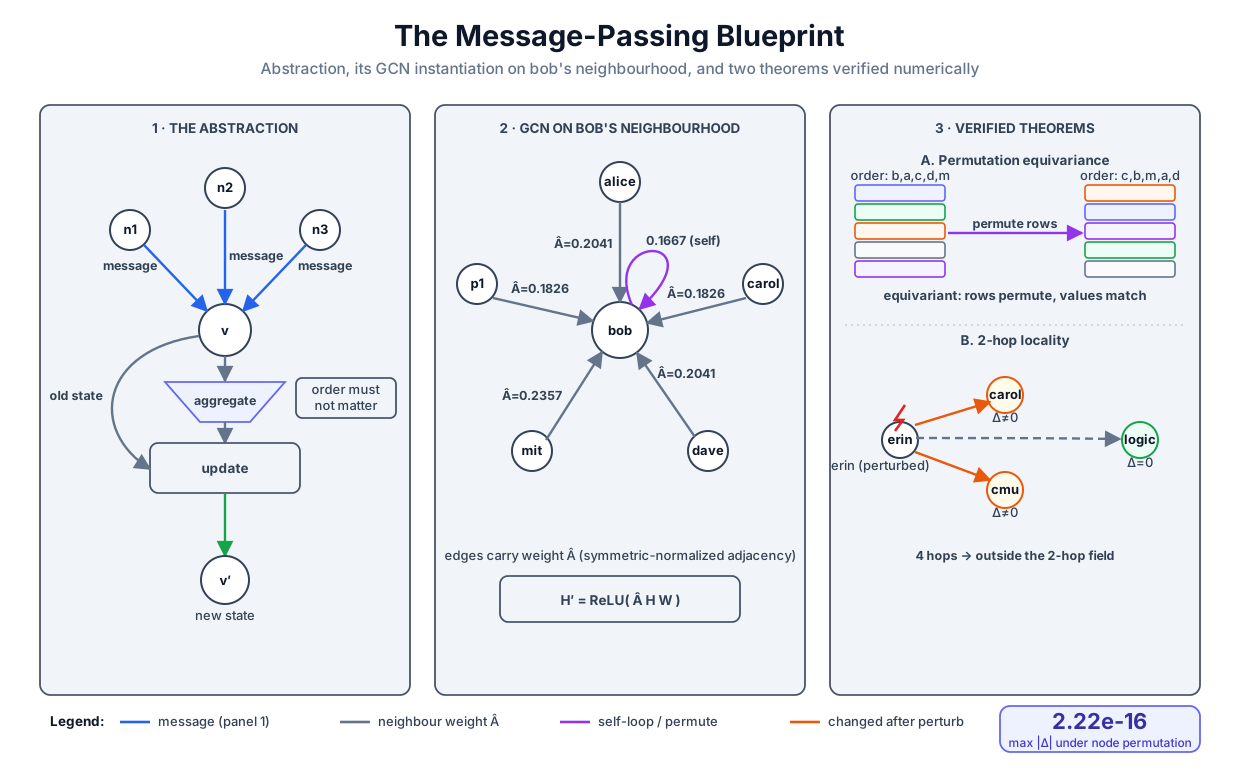The blueprint (message → aggregate → update), its GCN instantiation on bob's real neighborhood with the actual $\hat{A}$ weights, and the two theorems the trained network passes numerically: equivariance to float round-off and 2-hop locality, bitwise. Original diagram by the authors, created with AI assistance.

The graph as two matrices

The academic knowledge graph of kg.py has 13 entities and 18 triples. For this chapter we deliberately forget the relation labels: ('alice', 'advises', 'bob') and ('p2', 'cites', 'p1') both become plain undirected edges. The result is encoded in the adjacency matrix $A$, a table with one row and one column per node, in which the entry $A_{ij}$ (row $i$, column $j$) is $1$ if an edge joins nodes $i$ and $j$ and $0$ otherwise. Undirected means $A_{ij} = A_{ji}$, so $A$ is symmetric (equal to its own transpose, $A^\top = A$, where the transpose $\top$ flips a matrix across its diagonal). The companion file builds it in ten lines, five of them executable (gnn.py lines 56–65):

def build_adjacency() -> np.ndarray:
    """The 18 triples as an undirected, unlabelled adjacency matrix A
    (13 x 13, symmetric, zero diagonal).  Relation types are dropped on
    purpose: this module isolates pure message passing; ``rgcn.py`` adds
    relation-specific weights."""
    a = np.zeros((N, N))
    for h, _r, t in kg.TRIPLES:
        i, j = kg.E_ID[h], kg.E_ID[t]
        a[i, j] = a[j, i] = 1.0
    return a

The second matrix is the degree matrix $D$: the degree $d_i$ of node $i$ is its number of neighbors, the sum of row $i$ of $A$, and $D$ is the diagonal matrix with $d_1, \ldots, d_{13}$ down its diagonal and zeros elsewhere. On this graph the degrees range from 1 to 5: the topic nodes logic, ml, nesy each touch a single paper (degree 1), while bob, who advises two students, has an advisor, wrote a paper, and holds an affiliation, sits at degree 5. These two matrices are all the structure a GCN ever sees.

Why matrices at all? Because one matrix multiplication performs the entire message-passing round for every node at once. Stack the node vectors into a matrix $H$ whose row $i$ is $h_i^\top$ ($13 \times d$, one row per node). Then row $i$ of the product $AH$ is, by the definition of matrix multiplication,

$$(AH)_i \;=\; \sum_{j=1}^{13} A_{ij}\, h_j \;=\; \sum_{j \in \mathcal{N}(i)} h_j ,$$

since $A_{ij}$ is $1$ exactly on neighbors and $0$ elsewhere. Multiplying by $A$ is "sum the neighbors' vectors", executed for all 13 nodes in one shot. The blueprint's aggregate has become linear algebra. But this raw operator has two defects, and repairing them, one at a time, produces the GCN.

Assembling the layer: two defects, two repairs

Defect one: $A$ erases the node itself. The sum $\sum_{j \in \mathcal{N}(i)} h_j$ runs over the neighbors only; $A_{ii} = 0$, so $h_i$ contributes nothing to its own update. After one layer, a node's representation is built entirely from other nodes' features, and its own input feature is gone. The repair is a self-loop at every node: replace $A$ by $\tilde{A} = A + I$, where $I$ is the identity matrix (ones on the diagonal, zeros elsewhere). Now $\tilde{A}_{ii} = 1$, row $i$ of $\tilde{A}H$ is $h_i + \sum_{j \in \mathcal{N}(i)} h_j$, and every node stays inside its own receptive field [3].

Defect two: the sum scales with degree. Suppose every node's vector has roughly the same length $c$ (write $\lVert h_j \rVert \approx c$, where $\lVert \cdot \rVert$ is the Euclidean norm, the square root of the sum of squared components). Then the aggregated row for node $i$ is a sum of $d_i + 1$ such vectors, and if the summands are roughly aligned, as entrywise-nonnegative vectors such as our one-hot inputs and post-ReLU activations are, its length is on the order of $(d_i + 1)\,c$ (a sum of vectors in unrelated random directions would grow only like $\sqrt{d_i + 1}\,c$; alignment is what makes the growth linear). Concretely, on our graph, bob (degree 5) receives a sum of 6 vectors while logic (degree 1) receives a sum of 2: after one layer bob's activations are about 3 times larger, after two layers about 9 times, and in general the disparity compounds geometrically with depth, like powers of the degree. Nothing about being well-connected makes a node 9 times more important; the scale is an artifact of counting. Worse, the blow-up is graph-global: repeated multiplication by $\tilde{A}$ amplifies any vector along the matrix's dominant eigenvector by its largest eigenvalue (a number $\lambda$ for which some nonzero vector $v$ satisfies $\tilde{A}v = \lambda v$; applying the matrix $T$ times scales that direction by $\lambda^T$), and for an adjacency-like matrix that top eigenvalue grows with the graph's connectivity, so deep stacks explode along the dominant eigendirection, faster the denser the graph, while the components along eigenvalues smaller than $1$ in magnitude decay: an uncontrolled mix of blow-up and wash-out.

The repair is normalization, and the specific choice matters. Divide each entry by the degrees at both endpoints, symmetrically:

$$\hat{A} \;=\; D^{-1/2}\,\tilde{A}\,D^{-1/2}, \qquad\text{entrywise}\qquad \hat{A}_{ij} \;=\; \frac{\tilde{A}_{ij}}{\sqrt{d_i\, d_j}},$$

where, from here on, $d_i$ denotes the degree including the self-loop (row sums of $\tilde{A}$), and $D^{-1/2}$ is the diagonal matrix carrying $1/\sqrt{d_i}$. Each edge between nodes $i$ and $j$ (written $i \sim j$; the tilde is the standard shorthand for "$i$ and $j$ are adjacent") now carries weight $1/\sqrt{d_i d_j}$: a message is discounted once for the sender's popularity and once for the receiver's. Here is the claim that justifies it, with the argument in full.

Claim: every eigenvalue $\lambda$ of $\hat{A}$ satisfies $-1 \lt \lambda \le 1$. First compare $\hat{A}$ with the row-normalized walk operator $P_{\mathrm{rw}} = D^{-1}\tilde{A}$, whose entry $(P_{\mathrm{rw}})_{ij} = \tilde{A}_{ij}/d_i$ divides only by the receiver's degree, so every row of $P_{\mathrm{rw}}$ sums to exactly $1$. (The subscript rw abbreviates random walk, and it is there to keep the bare letter $P$ free: later sections give that letter two other standard jobs, the network's output probability matrix and the permutation matrix of theorem one.) The two are similar matrices: $\hat{A} = D^{-1/2}\tilde{A}D^{-1/2} = D^{1/2}\,(D^{-1}\tilde{A})\,D^{-1/2} = D^{1/2} P_{\mathrm{rw}} D^{-1/2}$, and similar matrices have identical eigenvalues (if $P_{\mathrm{rw}}v = \lambda v$ then $\hat{A}(D^{1/2}v) = D^{1/2}P_{\mathrm{rw}}v = \lambda\,(D^{1/2}v)$). So it suffices to bound the eigenvalues of $P_{\mathrm{rw}}$. Take any eigenvalue $\lambda$ of $P_{\mathrm{rw}}$ with eigenvector $v$, and let $i$ be the index where $\lvert v_i \rvert$, the absolute value of the entry $v_i$ (its magnitude with the sign dropped), is largest. Reading off row $i$ of $P_{\mathrm{rw}}v = \lambda v$ and splitting out the diagonal term:

$$\lambda\, v_i \;=\; \sum_{j} (P_{\mathrm{rw}})_{ij}\, v_j \;=\; (P_{\mathrm{rw}})_{ii}\, v_i + \sum_{j \ne i} (P_{\mathrm{rw}})_{ij}\, v_j .$$

Move the diagonal term across and bound the remainder using $\lvert v_j \rvert \le \lvert v_i \rvert$ and $(P_{\mathrm{rw}})_{ij} \ge 0$:

$$\lvert \lambda - (P_{\mathrm{rw}})_{ii} \rvert \, \lvert v_i \rvert \;=\; \Big\lvert \sum_{j \ne i} (P_{\mathrm{rw}})_{ij}\, v_j \Big\rvert \;\le\; \sum_{j \ne i} (P_{\mathrm{rw}})_{ij}\, \lvert v_j \rvert \;\le\; \Big( \sum_{j \ne i} (P_{\mathrm{rw}})_{ij} \Big) \lvert v_i \rvert \;=\; \big(1 - (P_{\mathrm{rw}})_{ii}\big)\, \lvert v_i \rvert,$$

where the last equality uses the row sum $\sum_j (P_{\mathrm{rw}})_{ij} = 1$. Dividing by $\lvert v_i \rvert \gt 0$ gives $\lvert \lambda - (P_{\mathrm{rw}})_{ii} \rvert \le 1 - (P_{\mathrm{rw}})_{ii}$, an interval centered at $(P_{\mathrm{rw}})_{ii}$ of radius $1 - (P_{\mathrm{rw}})_{ii}$, i.e. $2(P_{\mathrm{rw}})_{ii} - 1 \le \lambda \le 1$ (for the real eigenvalues at hand; $\hat{A}$ is symmetric, so all its eigenvalues are real). The self-loop makes the diagonal strictly positive, $(P_{\mathrm{rw}})_{ii} = 1/d_i \gt 0$, so the left end sits strictly above $-1$. Conclusion: $\lambda \in (-1, 1]$, and $\lambda = 1$ is attained (take $v$ with $v_i = 1$ everywhere: each row of $P_{\mathrm{rw}}v$ sums the row of $P_{\mathrm{rw}}$, which is $1$). Repeated application of $\hat{A}$ therefore never amplifies: the component along the top eigenvector is preserved ($1^T = 1$), and every other spectral component shrinks. (One caveat the interval alone does not settle: this needs the eigenvalue $1$ to be attained by exactly one direction, which holds on a connected graph, and ours is connected: a breadth-first search from any node reaches all 13. On a disconnected graph each connected piece would preserve one component of its own.) Hubs cannot blow up, deep stacks cannot explode, and the operator behaves the same on a graph of 13 nodes and a graph of 13 million.

Why the symmetric version rather than $P_{\mathrm{rw}}$ itself, since they share a spectrum? Two working reasons. First, $P_{\mathrm{rw}}$ weights a message only by the receiver's degree, so a hub's outgoing message is never discounted for the hub's own popularity; the symmetric weight $1/\sqrt{d_i d_j}$ splits the discount between both endpoints, damping traffic into and out of hubs. Second, and decisive for this chapter, $\hat{A}$ is symmetric ($\hat{A}^\top = \hat{A}$), and that single fact will quietly simplify a line of the backpropagation derivation below. The companion file builds the operator in three lines (gnn.py lines 68–81, docstring elided):

    a_tilde = a + np.eye(len(a))                 # A + I
    d = a_tilde.sum(axis=1)                      # degrees of A + I
    # Elementwise: Â[i, j] = Ã[i, j] / sqrt(d_i · d_j).
    return a_tilde / np.sqrt(np.outer(d, d))

and the layer itself, with the shared weight matrix and the ReLU nonlinearity (short for rectified linear unit: the function $\operatorname{ReLU}(z) = \max(z, 0)$, applied to every entry separately), is the one-line blueprint $H' = \operatorname{ReLU}(\hat{A} H W)$ (gnn.py lines 149–152):

    z1 = a_hat @ x @ w1
    h1 = np.maximum(z1, 0.0)                     # ReLU, applied elementwise
    z2 = a_hat @ h1 @ w2
    return z1, h1, z2, softmax(z2)

Match the pieces to the blueprint: the message from $j$ to $i$ is $h_j$ scaled by $\hat{A}_{ij} = 1/\sqrt{d_i d_j}$; the aggregate is the sum that the matrix product performs, self-loop included; the update is the shared linear map $W$ followed by the ReLU. Note that layer 2 has no interior ReLU: its output $Z_2$ feeds the softmax classifier head directly, and the softmax is its nonlinearity (the docstring at gnn.py lines 144–148 records what happens if you add one anyway: every logit gets clamped non-negative, most gradients gate to zero, and training stalls at 6 of 9 training labels). Here is the operator on real numbers: bob's row of $\hat{A}$, from the committed run. Bob's lifted degree is $5 + 1 = 6$, so his self-loop weighs $1/6 \approx 0.1667$; mit has lifted degree 3, so that edge weighs $1/\sqrt{6 \cdot 3} = 1/\sqrt{18} \approx 0.2357$; carol and p1 (lifted degree 5) weigh $1/\sqrt{30} \approx 0.1826$ each.

  A_hat = D^-1/2 (A+I) D^-1/2; nonzeros of bob's row: alice 0.2041, bob 0.1667, carol 0.1826, dave 0.2041, mit 0.2357, p1 0.1826

Features that force the network to read structure

A GNN needs an input feature matrix $X$, one row per node, and the choice is a scientific decision, not a formality. The obvious choice, a one-hot identity feature (row $i$ has a $1$ in position $i$), would sabotage the experiment: it hands each node a private input channel, so the weight matrix can simply memorize "channel 3 means Student" for each labeled node, and nothing learned would say anything about graph structure. The companion file's docstring states the choice and the reason (gnn.py lines 84–92; the full function runs through line 98):

def build_features(a: np.ndarray) -> tuple[np.ndarray, list[int]]:
    """X = one-hot of node DEGREE (13 x 5: the degrees present are 1..5).

    Structural features only, no identity features: a one-hot *node id* would
    hand each labelled node a private input channel, the weights would simply
    memorize the 9 training labels, and nothing learned would transfer to the
    held-out nodes.  Degree forces the model to generalize from structure
    alone (nodes of equal degree start indistinguishable and are separated
    only by their neighbourhoods)."""

So $X$ is $13 \times 5$: the degrees present on this graph are $1, 2, 3, 4, 5$, and each node's feature is the one-hot indicator of its own degree. Every degree-3 node (alice, cmu, dave, p3: a Professor, an Institution, a Student, and a Paper) starts with the identical input vector. If the network tells them apart at all, it can only be because message passing mixed in their neighborhoods.

The task is semi-supervised node classification [3]: every node's vector is computed, but the training loss reads the labels of only 9 of the 13 nodes. The other four, one per ambiguous type (gnn.py line 48: HELD_OUT: list[str] = ["bob", "dave", "p2", "cmu"]), are never labeled during training; the network still computes outputs for them on every forward pass, because they sit in the same graph and their features flow through $\hat{A}$ into everyone else. Predicting them correctly is the test of generalization. The committed setup line:

  split     : 9 labelled nodes for training; held out: bob (Professor), dave (Student), p2 (Paper), cmu (Institution)

Backpropagation through the stack, derived in full

The forward pass is three equations. With $W_1 \in \mathbb{R}^{5 \times 16}$ (input width 5, hidden width 16, set at gnn.py line 50) and $W_2 \in \mathbb{R}^{16 \times 5}$ (hidden width to the $C = 5$ classes):

$$Z_1 = \hat{A} X W_1, \qquad H_1 = \operatorname{ReLU}(Z_1), \qquad Z_2 = \hat{A} H_1 W_2, \qquad P = \operatorname{softmax}(Z_2),$$

where the softmax turns each row of logits $z = (z_1, \ldots, z_C)$ into a probability distribution, $p_k = e^{z_k} / \sum_{j=1}^{C} e^{z_j}$ (each entry positive, the row summing to 1). The loss is the masked cross-entropy: with $m = 9$ labeled nodes and $y_i$ the true class index of node $i$,

$$L \;=\; -\frac{1}{m} \sum_{i \,\in\, \text{labeled}} \ln p_{i, y_i},$$

the average negative log-probability the network assigns to the right answer (stated in the docstring at gnn.py lines 160–161, computed at line 172). Training is full-batch gradient descent, $W \leftarrow W - \eta\, \partial L/\partial W$: here $\partial L/\partial W$ is the matrix of partial derivatives of the loss with respect to each entry of a weight matrix $W$ (the symbol $\partial$ marks a derivative taken with all other variables held fixed), and $\eta$ is the learning rate, the step size of each update, set to $0.5$ (the lr=0.5 of the trace below; gnn.py line 51). So everything reduces to computing two gradient matrices. We work backwards from the loss, exactly as Gradient Descent did for the single neuron, and the first step reproduces that chapter's miracle in softmax form.

Step 1: the $p - y$ rule. Fix one labeled node and drop the node index; let $c$ be its true class, $y$ the one-hot target ($y_c = 1$, all other $y_k = 0$), and $z$ its logit row. Substitute the softmax into the loss and simplify before differentiating:

$$\ell \;=\; -\ln p_c \;=\; -\ln \frac{e^{z_c}}{\sum_{j} e^{z_j}} \;=\; -z_c + \ln \sum_{j} e^{z_j},$$

using $\ln(a/b) = \ln a - \ln b$ and $\ln e^{z_c} = z_c$. Now differentiate with respect to an arbitrary logit $z_k$. The first term contributes $-1$ if $k = c$ and $0$ otherwise, which is exactly $-y_k$. For the second term, the chain rule on $\ln(\cdot)$ gives one over the argument, times the argument's derivative; only the $j = k$ summand depends on $z_k$, and its derivative is $e^{z_k}$:

$$\frac{\partial \ell}{\partial z_k} \;=\; -y_k + \frac{1}{\sum_{j} e^{z_j}} \cdot e^{z_k} \;=\; -y_k + p_k \;=\; p_k - y_k .$$

The awkward normalizer differentiated into precisely the softmax itself, and the error signal collapses to probability minus target, the multi-class twin of the sigmoid result derived in Volume 1. Stacking this over nodes, averaging over the $m$ labeled ones, and zeroing the unlabeled rows with the mask gives the matrix

$$\Delta_2 \;=\; \frac{\partial L}{\partial Z_2} \;=\; \frac{1}{m}\,\operatorname{mask} \odot (P - Y),$$

where $Y$ is the one-hot label matrix and $\odot$ marks entrywise (row-wise, here) multiplication. That is gnn.py line 190: delta2 = (p - y_onehot) * train_mask[:, None] / m.

Step 2: the transpose, derived. The logits are a linear map of the aggregated hidden states: $Z_2 = M W_2$ with $M = \hat{A} H_1$. We need $\partial L/\partial W_2$, and the clean way is to differentiate one scalar entry. Entry $(i, k)$ of the product is $(Z_2)_{ik} = \sum_{c} M_{ic}\, (W_2)_{ck}$, so the derivative of $(Z_2)_{ik}$ with respect to a particular weight $(W_2)_{ab}$ is $M_{ia}$ when $k = b$ (the single term $c = a$ survives) and $0$ when $k \ne b$ (no term contains that weight). Summing the chain rule over every path from $(W_2)_{ab}$ to the loss:

$$\frac{\partial L}{\partial (W_2)_{ab}} \;=\; \sum_{i, k} \frac{\partial L}{\partial (Z_2)_{ik}} \frac{\partial (Z_2)_{ik}}{\partial (W_2)_{ab}} \;=\; \sum_{i} (\Delta_2)_{ib}\, M_{ia} \;=\; \sum_{i} (M^\top)_{ai}\, (\Delta_2)_{ib} \;=\; \big(M^\top \Delta_2\big)_{ab} .$$

The transpose is not a convention; it is what the index bookkeeping produces: the sum runs over the node index $i$, which is the row index of both $M$ and $\Delta_2$, and contracting two matrices along their shared row index is by definition $M^\top \Delta_2$. Hence

$$\frac{\partial L}{\partial W_2} \;=\; (\hat{A} H_1)^\top\, \Delta_2 ,$$

which is gnn.py line 194: grad_w2 = (a_hat @ h1).T @ delta2.

Step 3: back through the aggregation. Now view $Z_2 = \hat{A} H_1 W_2$ as a function of $H_1$, the middle factor of a three-matrix product. This is a genuinely different bookkeeping problem from step 2, because the middle factor is contracted on both sides at once: entry $(i, k)$ of the logits is $(Z_2)_{ik} = \sum_{v} \sum_{c} \hat{A}_{iv}\, (H_1)_{vc}\, (W_2)_{ck}$, summed over the node index $v$ and the hidden index $c$. Differentiating with respect to one hidden entry $(H_1)_{ab}$ kills every summand except the one with $v = a$ and $c = b$, leaving $\partial (Z_2)_{ik} / \partial (H_1)_{ab} = \hat{A}_{ia}\, (W_2)_{bk}$, and the chain rule sums over every logit entry:

$$\frac{\partial L}{\partial (H_1)_{ab}} \;=\; \sum_{i, k} (\Delta_2)_{ik}\, \hat{A}_{ia}\, (W_2)_{bk} \;=\; \sum_{i} (\hat{A}^\top)_{ai} \sum_{k} (\Delta_2)_{ik}\, (W_2^\top)_{kb} \;=\; \big(\hat{A}^\top \Delta_2 W_2^\top\big)_{ab} .$$

Two contractions this time, not one: over the node index $i$ (through $\hat{A}$, giving the left transpose) and over the class index $k$ (through $W_2$, giving the right transpose). Hence $\partial L/\partial H_1 = \hat{A}^\top \Delta_2 W_2^\top$, and here the symmetric normalization pays its second dividend: $\hat{A}^\top = \hat{A}$, so the backward pass reuses the forward operator unchanged (gnn.py lines 196–197). The gradient, like the activations, flows along the graph's edges: a labeled node's error signal propagates to its neighbors' hidden states through the same degree-weighted wiring.

Step 4: the ReLU gate. $H_1 = \max(Z_1, 0)$ entrywise, so each entry of $H_1$ has derivative $1$ with respect to its own $Z_1$ entry where $Z_1 \gt 0$, and $0$ where $Z_1 \lt 0$ (the function is flat to the left of zero). At exactly $Z_1 = 0$ the two slopes disagree and no derivative exists; the implementation adopts the standard convention of taking $0$ there, which the strict inequality in (z1 > 0.0) encodes. The chain rule multiplies the incoming gradient by this indicator: $\partial L/\partial Z_1 = (\partial L/\partial H_1) \odot \mathbf{1}[Z_1 \gt 0]$, which is gnn.py line 201: d_z1 = d_h1 * (z1 > 0.0). Gradients pass through active units untouched and die at inactive ones.

Step 5: the first weights. $Z_1 = (\hat{A} X) W_1$ has exactly the shape of step 2 with $M = \hat{A}X$ and $\Delta_1 = \partial L/\partial Z_1$, so $\partial L/\partial W_1 = (\hat{A} X)^\top \Delta_1$ (gnn.py line 204), and the update $W \leftarrow W - \eta\, \nabla_W L$ closes the loop (gnn.py lines 207–208); the symbol $\nabla_W L$ (read "nabla") is the gradient with respect to $W$, the same matrix of partial derivatives $\partial L/\partial W$ in a more compact notation. Five steps, two gradient matrices, no autograd. Running the file (seed 0, 400 epochs) prints the committed trace:

training: full-batch GD, lr=0.5, hidden width 16, 400 epochs, seed 0
  untrained loss = 1.5950  (uniform guessing over 5 classes would give ln 5 = 1.6094)
  epoch    loss   train-acc
      1  1.5690   0.3333
     50  0.8099   0.7778
    100  0.4853   1.0000
    200  0.2211   1.0000
    400  0.0845   1.0000

Read the first line as a sanity anchor: an untrained network should know nothing, and a uniform guess over $C = 5$ classes assigns probability $1/5$ to the truth, for a loss of $-\ln(1/5) = \ln 5 \approx 1.6094$; the random initialization lands at $1.5950$, essentially there. The trace then falls monotonically, crosses full training accuracy by epoch 100, and settles at $0.0845$:

epoch	loss $L$	train accuracy
0 (untrained)	1.5950	—
1	1.5690	3/9 = 0.3333
50	0.8099	7/9 = 0.7778
100	0.4853	9/9 = 1.0000
200	0.2211	9/9 = 1.0000
400	0.0845	9/9 = 1.0000

Fitting 9 labels is not the achievement; a big enough network can fit anything. The achievement, and the reason to trust the machinery, is what the same trained network does next: it passes two structural theorems and then generalizes to the nodes it never saw labeled.

Theorem one: permutation equivariance, exact to round-off

Node indices are bookkeeping. Whether alice is row 0 or row 11 of the matrices is a storage decision, and a function of the graph must not care. The formal statement uses a permutation matrix $P$: pick a reordering $\pi$ of the 13 indices and let $P$ have a $1$ in position $(i, \pi(i))$ and zeros elsewhere, so that row $i$ of $PX$ is row $\pi(i)$ of $X$ (the rows shuffled by $\pi$), and $PAP^\top$ shuffles both the rows and the columns of $A$, relabeling the same graph. (A warning about the letter: throughout this section $P$ is this permutation matrix, matching the companion code's exhibit output; it is unrelated to the probability matrix $P = \operatorname{softmax}(Z_2)$ of the training section and to the walk operator $P_{\mathrm{rw}}$ of the eigenvalue argument.) Writing $f(A, X)$ for the whole trained network's output matrix, the property is equivariance (not invariance: the output is a per-node matrix, so it should shuffle along with the input rather than stay fixed):

$$f(P A P^\top,\, P X) \;=\; P\, f(A, X).$$

The proof is a chain of three observations, each one line. First, the normalization commutes with relabeling: the lifted matrix is $PAP^\top + I = P(A + I)P^\top$ (because $PIP^\top = PP^\top = I$; a permutation matrix's inverse is its transpose), its degree vector is the old one shuffled (row sums are preserved under column permutation), so $D' = PDP^\top$; and since conjugating a diagonal matrix by a permutation merely reorders its diagonal entries, taking the entrywise inverse square root commutes with that reordering, $(PDP^\top)^{-1/2} = P D^{-1/2} P^\top$. Hence

$$\hat{A}' \;=\; (PDP^\top)^{-1/2}\, P(A+I)P^\top\, (PDP^\top)^{-1/2} \;=\; P D^{-1/2} \underbrace{P^\top P}_{I} (A+I) \underbrace{P^\top P}_{I} D^{-1/2} P^\top \;=\; P \hat{A} P^\top .$$

Second, the linear layer commutes: $\hat{A}'\,(PX)\,W_1 = P\hat{A}P^\top P X W_1 = P\,(\hat{A}XW_1) = PZ_1$, using $P^\top P = I$ again; the crucial structural fact is that $W_1$ is shared across nodes, multiplying on the feature side, so it never touches the node index. Third, ReLU acts entrywise and softmax acts row-wise, so both commute with any row shuffle. Composing through layer 2, every intermediate quantity of the permuted run is the $P$-shuffle of the original run, and the claim follows. No architecture that indexed nodes individually (a per-node bias, an identity feature) would survive this argument, which is exactly why the blueprint forbids them.

The companion file does not stop at the argument; it executes it on the trained network (gnn.py lines 282–292): draw a seeded permutation, rebuild $\hat{A}$ from the relabeled graph, rerun the same trained weights on $(PAP^\top, PX)$, and compare against $P\,f(A, X)$:

exhibit 1 — permutation equivariance: f(P A P^T, P X) = P f(A, X)
  seeded permutation P: [11, 9, 5, 6, 2, 7, 8, 1, 12, 4, 3, 10, 0]
  max |f(P A P^T, P X) - P f(A, X)| = 2.22e-16  (pure float round-off)

The largest absolute discrepancy across all $13 \times 5$ output probabilities is $2.22 \times 10^{-16}$, one unit in the last place of a double-precision number near 1, which is what "equal, up to reordering the same additions" looks like in floating point. The harness asserts it below $10^{-9}$ (gnn.py line 319); it passes with more than six orders of magnitude to spare.

Theorem two: 2-hop locality, verified bitwise

The second theorem bounds what a node can see. Unroll the two layers as one expression:

$$Z_2 \;=\; \hat{A}\, \operatorname{ReLU}\!\big(\hat{A} X W_1\big)\, W_2 .$$

Read the output row of a node $u$ from the outside in. The outer multiplication gives $(Z_2)_u = \sum_{v} \hat{A}_{uv} (H_1)_v W_2$, and $\hat{A}_{uv} \ne 0$ only when $v$ is $u$ itself or a direct neighbor: one hop. Each contributing hidden row is $(H_1)_v = \operatorname{ReLU}\big(\sum_{w} \hat{A}_{vw}\, X_w W_1\big)$, and $\hat{A}_{vw} \ne 0$ only when $w$ is in $v$'s closed neighborhood: a second hop. ReLU and softmax act within a row and never mix rows. So the output at $u$ is a function of exactly the input rows $X_w$ with $w$ at hop distance at most 2 from $u$, and of nothing else. A $T$-layer GCN sees a $T$-hop ball; this is its receptive field, and it is a theorem, not a tendency.

Theorems of the form "depends on nothing else" invite the strongest possible test: not "changes little" but "changes at all". The companion file picks the pair logic and erin, verifies by breadth-first search that they are 4 hops apart (logic's only neighbor is p1; the shortest path runs logic–p1–p2–carol–erin), then adds $10^6$ to every feature of erin and reruns the trained forward pass (gnn.py lines 298–316):

exhibit 2 — locality: a 2-layer GCN sees exactly 2 hops
  BFS distance logic <-> erin = 4 hops (more than 2)
  perturb X[erin] by +1e6 in every feature, rerun the trained forward pass:
  max |change in output(logic)|  = 0.0000000000   (bit-identical)
  max |change in output| over erin's neighbours ['carol', 'cmu'] = 0.9871

The far node's output moves by exactly $0.0$, and the harness asserts equality, diff_far == 0.0, not approximate closeness (gnn.py line 321). This exactness is worth a moment. The dense matrix products do consume erin's perturbed row even while computing logic's output, but only multiplied by an $\hat{A}$ coefficient that is exactly zero: a row outside logic's closed 2-hop ball enters its dot products with weight $0.0$, and $0.0$ times any finite value is exactly $0.0$ in floating point. Every partial sum along the way is therefore built from bit-identical terms added in the identical order in both runs, and deterministic floating-point arithmetic then produces bit-identical outputs. Meanwhile the perturbation does land where the theorem permits: erin's direct neighbors carol and cmu see their output probabilities shift by up to $0.9871$, a near-total flip. The receptive-field claim is made bitwise: inside the ball, nearly everything; outside it, nothing.

The held-out verdict, honestly read

Now the generalization test. The trained network's predictions on the four nodes whose labels it never saw, from the committed run:

held-out predictions (never labelled during training):
  node   true          predicted     correct?
  bob    Professor     Professor     yes
  dave   Student       Student       yes
  p2     Paper         Paper         yes
  cmu    Institution   Student       NO
  held-out accuracy: 3/4 = 0.7500   (train accuracy 1.0000)

node	true type	predicted	correct
bob	Professor	Professor	yes
dave	Student	Student	yes
p2	Paper	Paper	yes
cmu	Institution	Student	no

Three of four, from features that encode nothing but a degree count. Remember what the network had to overcome: dave starts with the same input vector as alice (Professor), cmu (Institution), and p3 (Paper), all degree 3; whatever separates them was assembled entirely by two rounds of $\hat{A}$, that is, from the degree profiles of their neighborhoods and their neighborhoods' neighborhoods. That is structure alone carrying the prediction, which is precisely the point the feature choice was engineered to make.

The error is as instructive as the successes. The only labeled Institution is mit: a degree-2 node whose two neighbors (alice, bob) have degrees 3 and 5. That is the entire structural definition of "Institution" available at training time. But cmu presents a different profile: degree 3, with neighbors carol, dave, erin of degrees 4, 3, 2, exactly the profile of a well-connected member of the student cluster; indeed it is structurally close to dave (degree 3, neighbors of degrees 5, 3, 3). Degree-only features give the network no way to know that being affiliated-to is what unifies mit and cmu, because the operator $\hat{A}$ erased the edge label affiliated before training began. With one exemplar and no relation types, the network filed cmu with the students it is wired to, a reasonable inference from the evidence it was permitted to see. Degree-only features on this graph can separate classes whose neighborhood degree profiles differ within 2 hops (papers hang off authors and topics; professors sit atop advising fans); they cannot separate classes whose membership is defined by which kind of edge arrives, and Institution is such a class. The harness accepts the run at 3 of 4 (gnn.py line 324), recording the failure rather than tuning it away.

The unsolved part

The cmu failure is not an accident of this small graph; it is the visible symptom of a decision made in the very first code block. build_adjacency writes a[i, j] = a[j, i] = 1.0 for every triple, and at that moment advises, authored, cites, affiliated, and about all become the same wire. The operator $\hat{A}$ then propagates every message with a weight that depends only on degrees, never on what the edge means. But the academic graph is a knowledge graph precisely because its edges mean different things: an advises edge is evidence about people and rank, a cites edge is evidence about papers and lineage, an affiliated edge is the defining evidence for institutions. Collapsing them throws that meaning away before learning begins, and no amount of training recovers information the input representation destroyed.

There is a deeper version of the question that this Part will keep circling. Message passing computes with local structural summaries, and we will see in The Expressiveness Ceiling that its discriminating power is exactly bounded by the Weisfeiler-Leman color-refinement test: two nodes whose neighborhood-degree unfoldings agree are, to a GCN with structural features, the same node. What is genuinely open is not whether the ceiling exists (that is a theorem) but how much of reasoning fits under it: which entailments of a symbolic system such as Volume 2's EL++ completion can be computed by any bounded-depth, permutation-invariant message passer at all, and which are forever out of local reach. The next chapter takes the first, concrete step: stop collapsing the wires.

Why it matters

For this volume, the blueprint is the second great representational move. Every model before this chapter embedded a graph into geometry and scored triples pointwise; this chapter made the graph itself the computation, and proved that the computation respects the two properties any function of a graph must have: indifference to node order and dependence only on actual connectivity. Those proofs, one algebraic and confirmed to $2.22 \times 10^{-16}$, one structural and confirmed bitwise, are a small model of the standard this series holds neural claims to: a property is not a slogan, it is an equation you can test.

For the neuro-symbolic road ahead, look again at what one GCN layer does: it holds a table of per-node assertions and extends each entry by combining the entries of its graph neighbors, repeatedly, layer by layer. Volume 2's completion algorithm did the same thing: it held the ledgers $S(A)$ and $R(r)$ and grew them by firing local rules along role edges until fixpoint. Message passing is, in a precise sense, a soft, differentiable cousin of rule application: bounded rounds instead of saturation, weighted sums instead of set union, gradients instead of derivations. That kinship is why GNNs are the neural half most often bolted to symbolic systems, and why their expressiveness ceiling matters so much: it delimits which rule-like inferences the soft cousin can even imitate. Volume 4 lives inside that gap.

Key terms

• Message passing — the layer scheme $h_i' = \operatorname{update}(h_i, \operatorname{aggregate}(\{\operatorname{message}(h_i, h_j) : j \in \mathcal{N}(i)\}))$; every GNN in this Part instantiates its three slots.
• Permutation invariance / equivariance — invariance: the output ignores input order (required of the aggregate over the neighbor multiset); equivariance: the output reorders along with the input, $f(PAP^\top, PX) = Pf(A, X)$ (satisfied by the whole network).
• Adjacency matrix $A$ / degree matrix $D$ — the graph as a 0-1 table of edges, and the diagonal matrix of neighbor counts; multiplying by $A$ sums each node's neighbors' vectors.
• Self-loop ($+I$) — the added diagonal that keeps a node's own state inside its update; without it, one layer erases every node's own features.
• Symmetric normalization $\hat{A} = D^{-1/2}(A+I)D^{-1/2}$ — each edge weighted $1/\sqrt{d_i d_j}$; all eigenvalues lie in the interval from above $-1$ up to $1$, so repeated application never amplifies, and $\hat{A}^\top = \hat{A}$ simplifies backpropagation.
• Semi-supervised node classification — training on the labels of a subset of nodes while every node's representation is computed in the same graph; the held-out nodes test structural generalization.
• The $p - y$ rule — the gradient of cross-entropy through softmax collapses to probability minus one-hot target, $\partial \ell/\partial z_k = p_k - y_k$.
• Receptive field — the $T$-hop ball a $T$-layer GNN's output provably depends on, and nothing outside it; verified here bitwise.

Where this leads

The chapter's one failure pointed at the chapter's one simplification: $\hat{A}$ has a single wire where the graph has five kinds of edges. The repair is as direct as the diagnosis. Give each relation $r$ its own weight matrix $W_r$, sum messages per relation and then across relations, and the update becomes $h_i' = \sigma\big(W_0 h_i + \sum_r \sum_{j \in \mathcal{N}_r(i)} \frac{1}{c_{i,r}} W_r h_j\big)$, where $\sigma$ is a nonlinearity applied entrywise (the ReLU, in the next chapter's implementation), $\mathcal{N}_r(i)$ is $i$'s neighborhood along relation $r$ alone, and $c_{i,r}$ is a per-relation normalizing count: a relational GCN, in which advises and cites finally travel on different wires and an affiliated edge can mean something no citation means. Whether that repair rescues cmu, what it costs in parameters, and what new failure it exposes is the business of the next chapter, Relational GNNs.

---

Companion code: examples/neural/gnn.py implements everything in this chapter with NumPy alone: the adjacency and the operator $\hat{A}$ (lines 56–81), the degree features (lines 84–98), the two-layer forward pass (lines 136–152), the hand-derived backpropagation (lines 184–208), and the two exhibits with their competency asserts (lines 279–324). Run python3 gnn.py from examples/neural/ to reproduce every number quoted above; the suite harness examples/neural/validate.py runs the same checks as part of the volume's acceptance verdict.