Link Prediction: Completing the Graph

📍 Where we are: Part I · Knowledge Graph Embeddings — Chapter 1. Volume 2 — The Honest Verdict closed with symbols that abstain on any fact they cannot prove; this chapter turns that abstention into a statistical question and builds the yardstick that will measure every answer in this volume.

Volume 2 ended on a deliberately uncomfortable note. Its reasoners were sound, complete, and fast, and they were also, by design, silent about anything the axioms did not entail. It called the open-world assumption principled abstention: a missing fact yields "not entailed," never "false" and never "probably." This chapter refuses to leave it at that. We take the same academic world, delete a fact we know is true, confirm that no amount of logic can bring it back, and then build the machinery that guesses it back: a score for every candidate fact, a sorted list, and two numbers, Mean Reciprocal Rank (MRR) and Hits@k, that say how close to the top the truth landed. No model is trained in this chapter. The protocol comes first, because it is the scoreboard for every link-prediction model in this volume, from Part I's translations through Part IV's relational graph neural networks.

The simple version

Imagine a streaming service that has seen you rate a handful of films. It cannot prove you will love a film you have never rated; there is no logical derivation from "liked these two" to "will like that one." What it can do is line up every film you have not seen, give each a plausibility score, and sort the line. If a film you genuinely would love lands in the top three, the guesser is good; at position eleven of thirteen, it is useless. Link prediction treats a knowledge graph's missing facts exactly this way: the held-out true fact is the film you would have loved, the scorer is the model, and the art of this chapter is measuring, fairly, where the truth lands in the sorted list.

What this chapter covers

• The missing edge no proof can reach: why Volume 2's reasoners, given every axiom, still cannot name whom bob advises beyond what was asserted, and why that failure is structural.
• The score function: completion reframed as ranking: a function $s(h, r, t)$ mapping any candidate triple to a real number, with order the only thing that matters.
• The data, exactly: the 18 triples of kg.py, imported from Volume 1's facts rather than retyped, and the deterministic 15/3 split whose invariants are enforced by assert.
• The filtered ranking protocol, derived: raw versus filtered ranks, why other known-true answers leave the candidate list, how ties are counted, and the exact definitions of MRR and Hits@k.
• What chance earns: a full derivation of the random baseline's expected MRR from harmonic numbers, and the committed frozen-random numbers that make "better than nothing" measurable.
• A first trained result: the committed output of transe.py as a teaser: learning moves the metric from 0.1062 to 0.7778 before we have even defined the model.
• Methodology honesty: leakage through the negative sampler, the tie-handling pathology, and why 6 queries is a demonstration while FB15k-237 and WN18RR are the field's scale.

The missing edge no proof can reach

Every volume of this series reads the same tiny academic world, and each reads it differently: Volume 1 as facts and Horn rules, Volume 2 as an EL++ ontology. Both readings share one discipline: a fact is either asserted, derived, or unknown, and unknown is a final answer. Delete advises(bob, carol) and the reasoner does not degrade to "probably still advises"; it simply stops entailing everything downstream and reports no error.

Now make the failure concrete. Suppose the curator forgot to record that bob advises dave. Volume 2's TBox does entail something relevant: from the axiom $\text{Professor} \sqsubseteq \exists \text{advises}.\text{Student}$, every professor advises some student, so the reasoner can prove that bob advises someone, some anonymous student. What it can never do is name that student. There is no axiom, and there could be no sound axiom, from which advises(bob, dave) follows and advises(bob, erin) does not; both are consistent with everything else written down. A derivation ends in an existential with no witness. The edge to dave is simply not in the deductive closure, and no reasoner, however complete, derives facts outside the closure. Completeness means "derives everything entailed," not "recovers everything true."

This is not a corner case; it is the normal condition of real knowledge graphs. Surveys of relational machine learning report that even the largest public knowledge graphs are missing enormous fractions of the basic facts about the entities they contain [1]. The missing facts were never derivable, because they are contingent facts about the world, not logical consequences of other facts. If we want them, we must change the question. Instead of asking "is this fact entailed?" (answer: no, and it never will be), we ask a statistical one: among all the edges the graph does not contain, which are likely true? That question has no proof-theoretic answer. It has a learnable one.

From derivation to ranking: the score function

The reframing takes one definition. Write $\mathcal{E}$ for the set of entities (the nodes of the graph; here 13 of them) and $\mathcal{R}$ for the set of relations (the edge types; here 5). A triple $(h, r, t)$ is a directed, labeled edge: a head entity $h$, a relation $r$, and a tail entity $t$, so advises(bob, dave) becomes $(\text{bob}, \text{advises}, \text{dave})$. A score function is any map

$$s : \mathcal{E} \times \mathcal{R} \times \mathcal{E} \;\to\; \mathbb{R},$$

read: $s$ takes a candidate triple, any head, any relation, any tail, and returns one real number ($\mathbb{R}$ is the set of real numbers), with the convention that a higher score means the model considers the triple more plausible. Nothing else about $s$ is fixed yet. It may come from geometry, from a bilinear form, from a neural network; every link-prediction model in this volume, from Part I's translations through Part IV's relational graph neural networks, is exactly a choice of $s$ plus a way to train it [2], [1]. (Parts II and III embed concepts and axioms as regions and judge them by their own membership and subsumption probes; whenever a model in this volume ranks candidate edges, this chapter's protocol is the judge.)

Link prediction (also called knowledge graph completion) is then the following task. A query is a triple with one entity masked: the tail query $(h, r, ?)$ asks "which entity does $h$ stand in relation $r$ to?", and the head query $(?, r, t)$ asks the converse. To answer a tail query, score every entity $e \in \mathcal{E}$ (read: each member $e$ of the entity set) as the candidate tail, giving 13 numbers $s(h, r, e)$, and sort them in descending order. The model's answer is not one entity; it is the whole ordering.

Notice what was traded away. Volume 2's answer to a query came with a derivation: a finite, auditable chain of rule firings, and a guarantee that the conclusion holds in every model of the axioms. The sorted list comes with neither. The score $s(\text{bob}, \text{advises}, \text{dave})$ is not a truth value, not a probability (nothing yet forces it into $[0,1]$ or calibrates it), and not the conclusion of any argument. It is a preference, meaningful only in comparison to the other candidates' scores. We gave up certainty and received, in exchange, the ability to say something at all about facts outside the deductive closure. The evaluation problem of this chapter is how to measure an ordering honestly; the modeling problem of the next several chapters is how to make the ordering good.

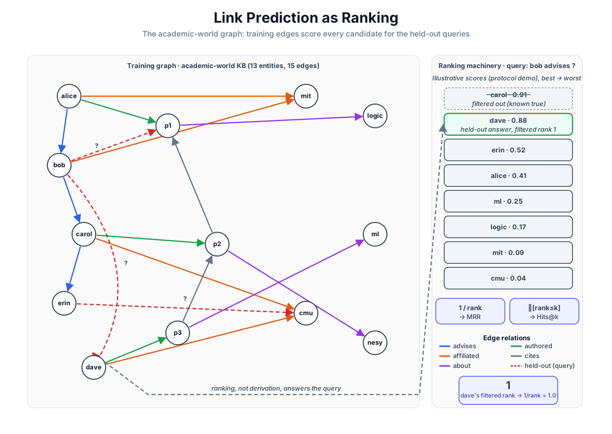Link prediction on the academic world: the training graph (solid edges) cannot derive the held-out dashed edges, so each becomes a ranking query; the candidate list is sorted by score, other known-true answers are filtered out, and the true answer's rank feeds MRR and Hits@k. Original diagram by the authors, created with AI assistance.

The data, exactly: 18 triples, a 15/3 split

Everything in this volume trains on one fixed dataset, defined once in examples/neural/kg.py and imported by every model. The triples are not retyped from memory; they are computed from Volume 1's kb.FACTS, so the three volumes provably share one world (kg.py lines 41–50):

def _binary_triples() -> list[tuple[str, str, str]]:
    """Every binary fact ``(pred, a, b)`` in ``kb.FACTS`` as an (h, r, t)
    triple.  Unary facts (``professor(alice)``) become *types*, not triples."""
    return [(f[1], f[0], f[2]) for f in FACTS if len(f) == 3]


TRIPLES: list[tuple[str, str, str]] = _binary_triples()

ENTITIES: list[str] = sorted({h for h, _, _ in TRIPLES} | {t for _, _, t in TRIPLES})
RELATIONS: list[str] = sorted({r for _, r, _ in TRIPLES})

Two reading notes. Volume 1 stored a binary fact as (predicate, arg1, arg2), so the comprehension reorders each fact into head-relation-tail form. And the unary facts, professor(alice) and its kin, do not become triples at all: in the knowledge-graph reading they are node types, kept in the TYPE_OF dictionary (from Volume 2's concept assertions) for the graph-neural-network chapters of Part IV. The derived relation grandAdvisor is absent by design: it is entailed by composing advises with itself, so asserting it as data would smuggle a derivable fact into the training set. Running python3 kg.py prints the inventory, the real committed output:

the academic world as a knowledge graph
  entities  (13): ['alice', 'bob', 'carol', 'cmu', 'dave', 'erin', 'logic', 'mit', 'ml', 'nesy', 'p1', 'p2', 'p3']
  relations (5): ['about', 'advises', 'affiliated', 'authored', 'cites']
  triples   : 18  (train 15 / test 3)
  test      : [('bob', 'advises', 'dave'), ('bob', 'authored', 'p1'), ('erin', 'affiliated', 'cmu')]
  types     : Institution = ['cmu', 'mit'], Paper = ['p1', 'p2', 'p3'], Professor = ['alice', 'bob'], Student = ['carol', 'dave', 'erin'], Topic = ['logic', 'ml', 'nesy']

So the graph has 13 entities (2 professors, 3 students, 3 papers, 2 institutions, 3 topics), 5 relations, and 18 edges, distributed like this:

relation	training edges (15)	held out for test (3)
advises	alice→bob, bob→carol, carol→erin	bob→dave
authored	alice→p1, carol→p2, dave→p3	bob→p1
affiliated	alice→mit, bob→mit, carol→cmu, dave→cmu	erin→cmu
cites	p2→p1, p3→p2	—
about	p1→logic, p2→nesy, p3→ml	—

The split itself is written out literally, not sampled, and its correctness is enforced the moment the module is imported (kg.py lines 65–74):

TEST: list[tuple[str, str, str]] = [
    ("bob", "advises", "dave"),
    ("bob", "authored", "p1"),
    ("erin", "affiliated", "cmu"),
]
TRAIN: list[tuple[str, str, str]] = [t for t in TRIPLES if t not in TEST]

assert len(TRIPLES) == 18 and len(TRAIN) == 15 and len(TEST) == 3
assert {h for h, _, _ in TRAIN} | {t for _, _, t in TRAIN} == set(ENTITIES)
assert {r for _, r, _ in TRAIN} == set(RELATIONS)

The last two assert lines are the split's design constraint, and they matter more than its size. The second asserts that every one of the 13 entities still occurs somewhere in the 15 training triples; the third asserts the same for all 5 relations. The reason is stated in the file's own comment: an embedding model cannot rank an entity it has never seen. The models of this volume are transductive: they learn one vector (or box, or ball) per known entity, so an entity absent from training would keep an arbitrary, untrained representation, and ranking it would measure noise. Each held-out triple therefore leaves both its entities and its relation with other training occurrences: bob remains an adviser of carol and an employee of mit, dave remains an author of p3 and an affiliate of cmu, and authored keeps three training edges. The test triples are missing edges, never missing nodes.

The filtered ranking protocol, derived

Now the measurement. Fix a scored query, say the tail query $(\text{bob}, \text{advises}, ?)$ whose held-out true answer is dave. The model produces 13 scores, and the natural statistic is the rank of the true answer: dave's position in the descending sort. Two details make the naive definition dishonest, and fixing them produces the standard protocol [2].

Detail one: other true answers. The graph already knows a second true tail for this query: $(\text{bob}, \text{advises}, \text{carol})$ is a training triple. Suppose the model has learned well and puts carol at position 1 and dave at position 2. Under the raw rank, dave's rank is 2: the model is penalized one full position for being right about carol, and a model that knew less about carol would score better on dave, which is perverse. The filtered rank repairs this by removing from the candidate list every candidate that forms a different known-true triple: carol is skipped, everything else stays, and dave's filtered rank is 1. Filtering never removes the query's own answer, only its true siblings. The known-true set used for filtering is all 18 triples, training and test alike, held in KNOWN (kg.py line 107).

Detail two: ties. Two candidates can score exactly equally. The suite defines the rank as 1 plus the number of candidates scored strictly higher, so ties count in the true entity's favour. Formally, writing $C(h, r)$ for the surviving candidate set of the query (all entities, minus the true answer itself, minus the filtered siblings), and $\lvert \cdot \rvert$ for the number of elements in a set,

$$\mathrm{rank}(t \mid h, r) \;=\; 1 \;+\; \bigl|\; \lbrace\, e \in C(h, r) \;:\; s(h, r, e) \gt s(h, r, t) \,\rbrace \;\bigr|.$$

Read it as: start at rank 1 (a perfect answer) and lose one position for every surviving competitor that strictly outscores the truth. The implementation is a direct transcription (kg.py lines 91–104, the body of rank_of):

    known = KNOWN if known is None else known
    h, r, t = triple
    true_score = score_fn(h, r, t)
    rank = 1
    for e in ENTITIES:
        if corrupt == "tail":
            cand = (h, r, e)
        else:
            cand = (e, r, t)
        if cand == triple or (cand in known and cand != triple):
            continue
        if score_fn(*cand) > true_score:
            rank += 1
    return rank

The continue line is the filter: it skips the true triple itself (the truth never competes against itself) and every other known-true candidate. The final if is the strict comparison that resolves ties optimistically. Corrupting the head instead of the tail (corrupt="head") builds candidates $(e, r, t)$ and measures the same thing from the other side.

Each of the 3 test triples yields two queries, one per direction, so the suite has 6 ranking queries, each yielding one rank. Two summary statistics compress the six ranks, computed in evaluate (kg.py lines 110–122):

def evaluate(score_fn, test: list[tuple[str, str, str]] | None = None) -> dict:
    """Filtered MRR and Hits@k over head- and tail-corruption of ``test``
    (default: the 3 held-out triples, i.e. 6 ranking queries)."""
    test = TEST if test is None else test
    ranks: list[int] = []
    for triple in test:
        ranks.append(rank_of(score_fn, triple, "tail"))
        ranks.append(rank_of(score_fn, triple, "head"))
    mrr = sum(1.0 / r for r in ranks) / len(ranks)
    hits = {k: sum(1 for r in ranks if r <= k) / len(ranks) for k in (1, 3, 10)}
    return {"ranks": ranks, "mrr": round(mrr, 4),
            "hits@1": round(hits[1], 4), "hits@3": round(hits[3], 4),
            "hits@10": round(hits[10], 4)}

In symbols, with $Q$ the set of queries ($\lvert Q \rvert = 6$ here) and $\mathrm{rank}_q$ the filtered rank of query $q$'s true answer:

$$\mathrm{MRR} \;=\; \frac{1}{\lvert Q \rvert} \sum_{q \in Q} \frac{1}{\mathrm{rank}_q}, \qquad \mathrm{Hits@}k \;=\; \frac{1}{\lvert Q \rvert} \sum_{q \in Q} \mathbf{1}\bigl[\mathrm{rank}_q \le k\bigr].$$

Decode both. The Mean Reciprocal Rank averages not the ranks but their reciprocals: rank 1 contributes $1$, rank 2 contributes $0.5$, rank 10 contributes $0.1$. The reciprocal makes the metric top-heavy on purpose: improving an answer from rank 2 to rank 1 gains $0.5$, while improving from rank 10 to rank 9 gains barely $0.011$, so MRR rewards putting the truth at or near the top, which is what a user of a completion system experiences. It lives just above $0$ and at most $1$, and $1$ means every query answered perfectly. Hits@k is blunter: $\mathbf{1}[\cdot]$ is the indicator function, equal to $1$ when the bracketed condition holds and $0$ otherwise, so Hits@k is the fraction of queries whose true answer landed in the top $k$. The suite reports $k = 1, 3, 10$, the trio that has become the field's convention [3].

What would chance earn? The random baseline, derived

Before any number can impress, we need to know what a scorer with no knowledge at all would earn. Here the small size of our graph stops being a convenience and becomes a trap: with 13 entities, a random guesser is not negligible, and we can compute exactly how not-negligible.

Model an ignorant scorer as one assigning each candidate an independent random score from a continuous distribution, so all orderings of a query's candidate list are equally likely and ties have probability zero. Let $m$ be the size of the query's filtered candidate pool, the true answer plus its surviving competitors. By symmetry, the true answer's rank is uniformly distributed over the positions $1, 2, \ldots, m$: each has probability $1/m$. The expected reciprocal rank follows in two steps. First write the expectation ($\mathbb{E}$, the probability-weighted average) as a sum over the equally likely positions $k$, writing $\Pr[\cdot]$ for the probability that the bracketed event occurs:

$$\mathbb{E}\!\left[\frac{1}{\mathrm{rank}}\right] \;=\; \sum_{k=1}^{m} \Pr[\mathrm{rank} = k]\cdot\frac{1}{k} \;=\; \sum_{k=1}^{m} \frac{1}{m}\cdot\frac{1}{k} \;=\; \frac{1}{m}\sum_{k=1}^{m}\frac{1}{k}.$$

The remaining sum is the $m$-th harmonic number $H_m = 1 + \tfrac12 + \tfrac13 + \cdots + \tfrac1m$, so

$$\mathbb{E}\!\left[\frac{1}{\mathrm{rank}}\right] \;=\; \frac{H_m}{m}, \qquad\text{and likewise}\qquad \Pr[\mathrm{rank} \le k] \;=\; \frac{k}{m} \quad (k \le m),$$

the second identity because exactly $k$ of the $m$ equally likely positions satisfy the condition. Now compute $m$ for each of the six queries. The pool contains the true answer plus every surviving competitor: 13 entities minus the filtered known-true siblings, so $m = 13$ minus the number of other known-true answers:

query	filtered siblings	pool $m$	$\mathbb{E}[1/\mathrm{rank}] = H_m/m$	$\Pr[\mathrm{rank} \le 10] = 10/m$
(bob, advises, ?)	carol	12	0.2586	0.8333
(?, advises, dave)	—	13	0.2446	0.7692
(bob, authored, ?)	—	13	0.2446	0.7692
(?, authored, p1)	alice	12	0.2586	0.8333
(erin, affiliated, ?)	—	13	0.2446	0.7692
(?, affiliated, cmu)	carol, dave	11	0.2745	0.9091

Averaging the fourth column, the expected MRR of pure chance on this graph is $1.5256 / 6 = 0.2543$ (the sum carries the unrounded values; the 4-decimal entries as printed total $1.5255$). Averaging the fifth, the expected Hits@10 is $4.8834/6 = 0.8139$ (rounded column sum: $4.8833$); and since $\Pr[\mathrm{rank} \le 1] = 1/m$, the expected Hits@1 is $0.0814$. Read those numbers and the case against "accuracy" makes itself. A scorer that knows nothing already lands the truth in the top ten about 81 percent of the time, because the top ten is most of a 13-entity pool; Hits@10 is nearly saturated before learning begins, and even the chance MRR is a quarter of the maximum. On a graph this small, any headline number is meaningful only as a distance above the chance line, which is why the companion code computes the chance line explicitly rather than assuming it is zero.

The suite's actual baseline is one concrete draw of ignorance: embeddings of the same shape a model would use, drawn from a fresh random generator and never trained, pushed through the same evaluate (transe.py lines 179–186):

def random_baseline() -> dict:
    """The "geometry before learning" number: same-shape embeddings from a
    fresh rng (seed 1), never trained, run through the same evaluation."""
    rng = np.random.default_rng(1)
    b = 6.0 / math.sqrt(D)
    ent = rng.uniform(-b, b, size=(len(ENTITIES), D))
    rel = rng.uniform(-b, b, size=(len(RELATIONS), D))
    return kg.evaluate(make_score_fn(ent, rel))

Its committed result (first row of the output quoted below) is MRR $= 0.1062$ with ranks $[10, 10, 12, 7, 10, 9]$: five of the six truths buried near the bottom of their pools, the sixth barely below the middle. Note the honest gap between this observed $0.1062$ and the derived expectation $0.2543$. Part of it is sampling: the frozen draw is a single sample of a random geometry, not an average over draws, and this seed lands low (its Hits@10 of $0.8333$, by contrast, sits almost exactly on the derived $0.8139$). Part of it is model mismatch: a random geometry is not exactly the independent-scores model derived above, since its six ranks are correlated across queries through the shared entity vectors, and a distance-based score does not treat all candidates symmetrically (the candidate equal to the query's own entity, for instance, sits systematically closer to the query point than an unrelated entity does). Both numbers tell the same story: chance already earns a visible score, and only the margin above it is evidence of learning.

A first trained result

The next chapter builds and derives the simplest embedding model there is; this chapter borrows only its scoreboard. The committed output of python3 transe.py, after training that model for 1000 epochs on the 15 training triples, reports both rows of the comparison and all six per-query ranks:

filtered ranking over 6 queries (3 test triples × tail/head)
  model            MRR    H@1    H@3    H@10   ranks
  random (seed 1)  0.1062 0.0000 0.0000 0.8333 [10, 10, 12, 7, 10, 9]
  TransE trained   0.7778 0.6667 1.0000 1.0000 [3, 3, 1, 1, 1, 1]
  per query (filtered rank, random → trained):
    (bob, advises, ?dave)        10 →  3
    (?bob, advises, dave)        10 →  3
    (bob, authored, ?p1)         12 →  1
    (?bob, authored, p1)          7 →  1
    (erin, affiliated, ?cmu)     10 →  1
    (?erin, affiliated, cmu)      9 →  1

Trace the trained MRR by hand from its ranks, exactly as evaluate computes it: the ranks $[3, 3, 1, 1, 1, 1]$ give reciprocals $\tfrac13 + \tfrac13 + 1 + 1 + 1 + 1 = \tfrac{14}{3} \approx 4.6667$, and dividing by the 6 queries yields $0.7778$. Hits@1 is $4/6 = 0.6667$, and Hits@3 and Hits@10 are $6/6 = 1.0$ because no rank exceeds 3. Every fact the graph was missing is now in the top three of its candidate list, from a model that never saw any of the three test triples.

The same output also shows the filter working on live data. Here is the committed ranking table for the query $(\text{bob}, \text{advises}, ?)$, every entity scored as the tail:

  rank  tail    score
     1  carol   -0.3681  * gold (train), filtered rank 1
     2  bob     -0.4794
     3  erin    -0.7101
     4  dave    -0.7409  * gold (test), filtered rank 3
     5  alice   -0.8321

The model's best tail is carol, which is correct: bob really does advise carol, in the training data. Under a raw protocol, carol's presence would push the held-out answer dave from rank 3 to rank 4, charging the model for its own correct knowledge. The filtered protocol skips carol when ranking dave (and dave when ranking carol), which is why the table reports dave's filtered rank as 3 while he sits fourth in the raw sort. That one line of output is the whole argument for filtering, run on real numbers [2].

Hold the celebration lightly. The two "rank 3" entries are the interesting residue: the model surfaced dave but did not put him first, and why a translation-based geometry struggles to make one relation vector carry alice→bob, bob→carol, bob→dave, and carol→erin at once is the next chapter's subject. The point of this teaser is narrower: the metric moved from $0.1062$ to $0.7778$, and everything between those two numbers is learning, measured by a protocol fixed before the model existed.

Methodology honesty: leakage, ties, and scale

A ranking protocol is easy to build and easier to corrupt. Three failure modes deserve names before we trust any number this protocol reports.

Leakage into training. The evaluation only measures generalization if the test triples influence training in no way at all. The obvious rule is that they must not appear as positive examples; TRAIN excludes them by construction. The subtler rule concerns negative sampling. Embedding models train by contrasting true triples against corrupted ones, and the sampler that generates corruptions must consult a list of known-true triples so that it never presents a true fact as a negative. The suite's sampler does exactly this (transe.py lines 119–125, with KNOWN_IDS built from all 18 triples at lines 51–52):

    h, r, t = pos
    side = int(rng.integers(2))  # 0 = corrupt the head, 1 = corrupt the tail
    while True:
        e = int(rng.integers(len(ENTITIES)))
        cand = (e, r, t) if side == 0 else (h, r, e)
        if cand not in KNOWN_IDS:
            return cand

The design choice hiding in KNOWN_IDS is that the truth check covers the test triples too. If it covered only the training set, a corruption of $(\text{bob}, \text{advises}, \text{carol})$ could produce $(\text{bob}, \text{advises}, \text{dave})$, the very fact we hold out, and the model would be explicitly trained to score its own test answer low. The held-out fact must be absent from both sides of the training signal: never a positive (that would be memorization) and never a negative (that would sabotage the measurement). At benchmark scale, where corruptions collide with test triples vanishingly rarely, implementations often check against training data only; on 13 entities the collision probability is far too large to ignore.

Leakage through the data itself. A split can be poisoned before any model runs. The classic case is a benchmark whose relation set contains near-inverses: if the training set says $(a, r, b)$ and the test set asks about $(b, r^{-1}, a)$, a trivial rule answers the test without learning anything. Exactly this flaw was found in the original FB15k and WN18 benchmarks, where inverse-relation pairs let a simple memorizer post state-of-the-art numbers; the repaired FB15k-237 exists because of that audit [4], and WN18RR was later built the same way for WordNet [3]. Our graph dodges the specific trap (none of the 5 relations is another's inverse, and the derived grandAdvisor is excluded), but the lesson generalizes: the evaluation measures the split as much as the model.

Ties and protocol drift. The strict-inequality rank counts ties in the truth's favour, which is harmless for continuous scores but exploitable in the degenerate limit: a scorer returning the same constant for every triple has no strictly-higher competitors, so every rank is 1 and its MRR is a perfect $1.0$. Real evaluations guard against this with randomized or expectation-based tie-breaking; our suite relies on its scores being continuous functions of random-initialized real vectors, where exact ties have probability zero. More broadly, the training protocol itself (how many negatives per positive, which loss function, how long the budget, how wide the hyperparameter search) moves reported numbers by margins comparable to whole modeling innovations: a re-evaluation that equalized exactly these choices found years-old models matching far newer ones [5].

Scale. Finally, the caveat that governs every number in this volume: 6 queries is a demonstration, not a benchmark. With so few queries, one rank flipping from 3 to 1 moves MRR by $0.11$; no confidence interval worth stating fits in a sample of six. The field's yardsticks are FB15k-237 (14,541 entities, 237 relations, about 20k test triples) and WN18RR (about 41k WordNet entities) [3], where the same protocol runs over tens of thousands of queries and a single MRR point is meaningful [4], [5]. Our graph buys something those benchmarks cannot: every rank in this volume can be traced to named entities and checked by hand against an ontology we fully understand. The trade is statistical power for transparency, made with eyes open.

The unsolved part

The protocol measures where the truth ranks; it does not, and cannot, say what a score means. When the trained model of the next chapter assigns $(\text{bob}, \text{advises}, \text{dave})$ the score $-0.7409$, that number carries no truth conditions, no probability, no derivation an auditor could replay, and no guarantee that transfers beyond the six queries we happened to ask. Volume 2's verdict chapter could point to a proof for every claim; this volume's first scoreboard can point to nothing but a sorted list. There is also a blindness built into the metric itself: MRR checks whether known-true answers rank high, but never whether the ordering respects what the ontology knows. A model could rank the topic logic as a plausible advisee of bob, an absurdity under Volume 2's TBox, and pay no metric penalty so long as dave ranks higher. Whether a geometry can be made to respect the schema, not just recall the edges, is the open thread Parts II and III pull on, and the honest admission here is that the yardstick we just built does not measure it at all.

Why it matters

Every link-prediction model in the coming chapters, from Part I's translations and bilinear forms to Part IV's relational graph neural networks, will be judged by the numbers defined here, on the same 6 queries, against the same chance line; the ranking habit itself, scoring candidates and measuring where truth lands, carries into the membership and subsumption probes of Parts II and III. Fixing the protocol before the first model is not pedantry; it is what makes the volume's comparisons mean something, and it mirrors how the field itself learned, through leaked benchmarks and drifting protocols, that evaluation discipline is as load-bearing as modeling insight [4], [5]. For the neuro-symbolic arc of this series, this chapter marks the exact point where the two traditions split and must eventually be rejoined: Volume 2 gave answers with proofs and abstained everywhere else; this chapter gives answers everywhere and proofs nowhere. Volume 4's differentiable query answering and Volume 5's soundness probes are, at bottom, attempts to buy back the guarantees traded away here, without giving up the ability to guess. You cannot appreciate that reconciliation without seeing the trade made nakedly, which is what the 15/3 split does.

Key terms

• Knowledge graph — entities connected by directed, labeled edges; each edge is a triple $(h, r, t)$ of head, relation, tail.
• Link prediction (knowledge graph completion) — ranking every candidate entity for a query $(h, r, ?)$ or $(?, r, t)$ by a learned score, to surface missing edges.
• Score function $s(h, r, t)$ — any map from candidate triples to real numbers, higher meaning more plausible; every link-prediction model is a choice of $s$.
• Corruption — replacing a triple's head or tail with another entity, to form an evaluation candidate or a training negative.
• Raw vs filtered rank — the truth's position among all candidates, versus its position after other known-true answers are removed; filtering stops a model being penalized for its own correct knowledge.
• MRR (Mean Reciprocal Rank) — the average of $1/\mathrm{rank}$ over all queries; top-heavy by design, $1.0$ is perfect.
• Hits@k — the fraction of queries whose true answer ranks in the top $k$; reported at $k = 1, 3, 10$.
• Chance line — the expected metric of an ignorant scorer; on a pool of $m$ candidates the expected reciprocal rank is $H_m/m$ with $H_m$ the $m$-th harmonic number, about $0.2543$ MRR here.
• Transductive split — a division in which every entity and relation still occurs in training, because a per-entity embedding model cannot represent what it never saw.
• Leakage — any path by which test information reaches training: test triples as positives, as sampled negatives, or structural giveaways such as inverse relations.

Where this leads

The scoreboard exists; the player does not. The gap left deliberately open is the score function itself: what geometry could make $s(\text{bob}, \text{advises}, \text{dave})$ large while keeping $s(\text{bob}, \text{advises}, \text{logic})$ small, using nothing but 15 observed edges? The next chapter, Translational Models, commits to the simplest possible answer: every entity becomes a point in $\mathbb{R}^{16}$, every relation a single translation vector, and a triple is plausible when $\mathbf{e}_h + \mathbf{w}_r$ lands near $\mathbf{e}_t$, so that $s(h, r, t) = -\lVert \mathbf{e}_h + \mathbf{w}_r - \mathbf{e}_t \rVert$, where $\lVert \cdot \rVert$ is the Euclidean length of the residual vector (derived in full next chapter). Deriving its margin loss and hand-computed gradients, and watching one shared advises vector strain to carry four different advising edges at once, is where the ranks $[3, 3, 1, 1, 1, 1]$ quoted above actually come from.

---

Companion code: examples/neural/kg.py defines the triples, the split, and the filtered-ranking evaluation used by every model in this volume; examples/neural/transe.py produced the baseline and trained numbers quoted here. Run python3 kg.py and python3 transe.py in examples/neural/ to reproduce every number in this chapter.