Hyperbolic Embeddings: Hierarchy in Curved Space

📍 Where we are: Part III · Embedding Ontologies — Chapter 11. TransBox and mOWL finished the toolbox for embedding EL++ axioms as regions in flat space; this chapter asks a more radical question: what if the space itself is the wrong shape for a hierarchy?

Every ontology embedding so far has changed the objects living in the space: points became boxes, balls, and translated regions, while the space underneath stayed $\mathbb{R}^d$, ordinary flat Euclidean space. But the deepest structure in the academic world, and in SNOMED CT, the Gene Ontology, and WordNet, is the is-a hierarchy, and a hierarchy is a tree. Trees have a growth rate that flat space simply cannot match: each generation multiplies the number of nodes, while a Euclidean ball's room grows only polynomially with its radius. This chapter makes that mismatch precise with a counting argument, then introduces a space whose room grows exponentially with radius, the Poincaré ball, decodes and differentiates its distance function, derives the Riemannian gradient descent that trains in it, and runs a committed head-to-head on the academic is-a tree at the same tiny dimension $d = 2$: same loss, same seed, same schedule, and only the geometry different.

The simple version

Imagine drawing your extended family tree on a round tabletop. You put the founding ancestor in the middle, the children in a ring around her, the grandchildren in a ring around them. Each ring must hold roughly twice as many people as the one before, but each ring is only a little longer than the one before, so by the fifth generation the names are overlapping and by the eighth they are unreadable. Now draw the same tree on a magic disc where rulers shrink as they slide toward the rim: a centimeter of table near the edge counts as a mile of "real" distance. Near the rim there is effectively unlimited room, so every generation gets a ring that is, in real distance, as roomy as it needs, forever. The Poincaré ball is that magic disc made mathematically exact, and training an embedding in it means doing gradient descent with the shrinking ruler taken into account at every step.

What this chapter covers

• The counting argument, done honestly: a $b$-ary tree has $b^k$ nodes at depth $k$; a packing bound shows a Euclidean ball of radius $k$ holds only polynomially many well-separated points, so flat embeddings of deep trees must pay in distortion or dimension; hyperbolic room grows like $e^{(d-1)r}$, the same rate as the tree.
• The Poincaré ball, decoded before the formula: the open unit ball with the metric factor $2/(1-\lVert\mathbf{x}\rVert^2)$ inflating distances near the boundary; the closed-form distance $d(\mathbf{u},\mathbf{v})=\operatorname{arcosh}\!\big(1+2\lVert\mathbf{u}-\mathbf{v}\rVert^2/((1-\lVert\mathbf{u}\rVert^2)(1-\lVert\mathbf{v}\rVert^2))\big)$ with every piece named, and worked checks at the center and at the rim.
• The distance differentiated: the full chain-rule derivation of $\partial d/\partial\mathbf{u}$, every algebraic step shown, landing exactly on the formula the companion code computes.
• Riemannian SGD (stochastic gradient descent) derived: steepest descent under the ball's own metric: the Euclidean gradient rescaled by $(1-\lVert\boldsymbol{\theta}\rVert^2)^2/4$, plus the projection guard that keeps every point inside the open ball.
• The committed head-to-head at $d=2$: the 22-node academic hierarchy embedded twice with identical loss, seed, negatives, and schedule; the ball wins the rank-correlation contest and sorts the tree radially, mean norm strictly increasing with depth.
• Why low dimension is the point: two dimensions let the chapter draw the true layout, and the field's result is that low-dimensional hyperbolic embeddings match far higher-dimensional Euclidean ones on hierarchies.
• Hyperbolic entailment cones: Part II's regions rebuilt inside curved space, closing the circle between geometry and subsumption.
• The unsolved part: every model so far embeds each node by table lookup; the graph's wiring deserves an encoder of its own, which opens Part IV.

The counting argument: trees outgrow flat space

Start with how fast a tree grows. In a $b$-ary tree, a tree in which every internal node has $b$ children (the letter $b$ is the branching factor), the root sits alone at depth $0$, its children at depth $1$ number $b$, their children number $b^2$, and in general depth $k$ (the letter $k$ counting generations from the root) holds $b^k$ nodes. Growth is exponential in depth: each extra generation multiplies the population. Even the modest academic hierarchy behaves this way at the leaves; its five generations run from one root to a deepest generation of six nodes (the concept Dean and five individuals), and a real ontology such as SNOMED CT runs a dozen generations deep over hundreds of thousands of concepts.

Now ask how much room flat space offers. Suppose we embed the tree so that every edge has length about $1$; then every node of depth at most $k$ lands inside a ball of radius $k$ around the root's image, and distinct nodes must stay some minimum distance apart, say at least $1$, or the embedding has collapsed them. So the real question is a packing question: how many points can sit inside a ball of radius $k$ in $\mathbb{R}^d$ (Euclidean space with $d$ coordinates, $d$ being the embedding dimension) while keeping every pairwise distance at least $1$?

The bound comes from comparing volumes, and every step is elementary. Let $\mathbf{x}_1,\ldots,\mathbf{x}_N$ be such points, $N$ of them (here and throughout, $\lVert\mathbf{a}\rVert$ is the ordinary Euclidean norm of a vector $\mathbf{a}$, its straight-line length, so $\lVert\mathbf{x}_i-\mathbf{x}_j\rVert$ is the straight-line distance between two of the points). Around each $\mathbf{x}_i$ draw a small ball $B(\mathbf{x}_i,\tfrac12)$ of radius $\tfrac12$. Two of these small balls cannot share an interior point: if some point $\mathbf{y}$ were inside both $B(\mathbf{x}_i,\tfrac12)$ and $B(\mathbf{x}_j,\tfrac12)$, the triangle inequality (the rule that a detour is never shorter than the direct path) would give $\lVert\mathbf{x}_i-\mathbf{x}_j\rVert \le \lVert\mathbf{x}_i-\mathbf{y}\rVert + \lVert\mathbf{y}-\mathbf{x}_j\rVert \lt \tfrac12+\tfrac12 = 1$, contradicting the separation. Each small ball also lies wholly inside the enlarged ball $B(\mathbf{0}, k+\tfrac12)$, since its center is within $k$ of the origin and its radius is $\tfrac12$. The volume of a radius-$R$ ball in $\mathbb{R}^d$ is $c_d R^d$ for a constant $c_d$ depending only on $d$, so $N$ disjoint balls of radius $\tfrac12$ fitting inside one ball of radius $k+\tfrac12$ forces

$$N \cdot c_d \left(\tfrac12\right)^{d} \;\le\; c_d \left(k+\tfrac12\right)^{d} \quad\Longrightarrow\quad N \;\le\; \left(\frac{k+\tfrac12}{\tfrac12}\right)^{d} \;=\; (2k+1)^{d}.$$

The capacity of flat space is polynomial in the radius: for fixed dimension $d$, a ball of radius $k$ holds at most $(2k+1)^d$ well-separated points. Set that against the tree's demand of $b^k$ nodes and take logarithms: a unit-edge, unit-separated embedding of depth $k$ needs $b^k \le (2k+1)^d$, that is,

$$d \;\ge\; \frac{k \ln b}{\ln(2k+1)},$$

a dimension that grows almost linearly with the depth of the tree. The concrete numbers make the squeeze vivid for a binary tree ($b=2$) in the plane ($d=2$):

depth $k$	tree nodes $2^k$	flat capacity $(2k+1)^2$	hyperbolic circumference $2\pi\sinh k$
$1$	$2$	$9$	$7.4$
$2$	$4$	$25$	$22.8$
$4$	$16$	$81$	$171.5$
$8$	$256$	$289$	$9365.0$
$16$	$65{,}536$	$1{,}089$	$\approx 2.8\times10^{7}$

By depth $8$ the binary tree has essentially consumed the plane, and by depth $16$ it demands sixty times more separated points than any radius-$16$ disc can hold. Something must give, and there are only two candidates: raise the dimension $d$ (parameters multiply), or let distances compress so that distinct nodes crowd together, which is distortion, a measured gap between graph distance and embedding distance. The trade-off between the two can be made exact, and the precise theorems say the same thing the packing bound sketches: flat space pays for trees, in dimension or in fidelity, and the price grows with depth [1].

The last column of the table is the escape route. In the hyperbolic plane, the two-dimensional space of constant negative curvature, the circumference of a circle of radius $r$ is not $2\pi r$ but $2\pi\sinh r$, where $\sinh r = (e^{r}-e^{-r})/2$ is the hyperbolic sine (its two siblings, used shortly, are the hyperbolic cosine $\cosh r = (e^{r}+e^{-r})/2$ and the hyperbolic tangent $\tanh r = \sinh r/\cosh r$); for large $r$ this is approximately $\pi e^{r}$, exponential in the radius. In $d$ dimensions hyperbolic volume grows like $e^{(d-1)r}$. A tree's population and a hyperbolic ball's room grow at the same rate, so a tree of any depth embeds in the hyperbolic plane with edges of honest length and nodes honestly separated: generation $k$ simply occupies the circle of radius proportional to $k$, whose length is exponentially large. Hyperbolic space is, in this exact sense, the continuous geometry of trees [2]. What remains is to build a computable model of it.

The Poincaré ball, decoded before the formula

The model we compute in is the Poincaré ball: as a set of points it is nothing exotic, just the open unit ball

$$\mathbb{B}^d \;=\; \{\, \mathbf{x} \in \mathbb{R}^d \;:\; \lVert\mathbf{x}\rVert \lt 1 \,\},$$

all vectors of Euclidean length less than one ("open" means the boundary sphere $\lVert\mathbf{x}\rVert = 1$ is excluded). What is exotic is the ruler. The ball carries a Riemannian metric, a rule assigning every point a local notion of length, and here the rule is conformal: at the point $\mathbf{x}$, every infinitesimal Euclidean length is multiplied by the factor

$$\lambda_{\mathbf{x}} \;=\; \frac{2}{1-\lVert\mathbf{x}\rVert^2},$$

the same factor in every direction (that direction-independence is what "conformal" means; as a matrix the metric is $g_{\mathbf{x}} = \lambda_{\mathbf{x}}^2 I$, a scalar times the identity). At the origin $\lambda = 2$, a fixed calibration constant. As $\lVert\mathbf{x}\rVert \to 1$ the denominator $1-\lVert\mathbf{x}\rVert^2$ goes to zero and $\lambda_{\mathbf{x}}$ blows up: near the rim, a hair's width of Euclidean motion is an enormous hyperbolic journey. The length of a path is the integral of $\lambda$ along it, and the distance between two points is the length of the shortest path (the geodesic) joining them. The rim itself is infinitely far from everywhere; the finite-looking disc contains an infinite world.

The exponential room promised above falls straight out of this factor. Take the circle of Euclidean radius $r$ centered at the origin. Its hyperbolic radius $\rho$ is the ruler-corrected distance from the center, and it can be computed directly from the metric. A straight radial segment is the shortest route from the center: any path $\mathbf{x}(s)$ from the origin to the point must move its norm from $0$ to $r$, the norm can change no faster than the path itself moves (the rate of change of $\lVert\mathbf{x}\rVert$ is the radial component of the velocity, at most its full length $\lVert\mathbf{x}'\rVert$), and the metric factor depends only on the norm, so every path's hyperbolic length is at least the radial integral below, which the radial segment attains. Evaluating that integral by partial fractions ($\tfrac{2}{1-t^2} = \tfrac{1}{1-t} + \tfrac{1}{1+t}$):

$$\rho(r) \;=\; \int_0^r \frac{2}{1-t^2}\,dt \;=\; \int_0^r\!\left(\frac{1}{1-t} + \frac{1}{1+t}\right)dt \;=\; \Big[\ln\frac{1+t}{1-t}\Big]_0^r \;=\; \ln\frac{1+r}{1-r} \;=\; 2\operatorname{artanh} r,$$

where $\operatorname{artanh}$ is the inverse hyperbolic tangent: solving $r = \tanh\rho' = (e^{2\rho'}-1)/(e^{2\rho'}+1)$ for $\rho'$ gives $e^{2\rho'} = (1+r)/(1-r)$, so $\operatorname{artanh} r = \tfrac12\ln\big((1+r)/(1-r)\big)$, matching the integral. Inverting, $r = \tanh(\rho/2)$. The circle's hyperbolic circumference is the metric factor at radius $r$ times its Euclidean circumference:

$$\lambda_r \cdot 2\pi r \;=\; \frac{2}{1-r^2}\cdot 2\pi r \;=\; 2\pi\cdot\frac{2r}{1-r^2} \;=\; 2\pi \cdot \frac{2\tanh(\rho/2)}{1-\tanh^2(\rho/2)} \;=\; 2\pi\cdot 2\sinh\!\big(\tfrac{\rho}{2}\big)\cosh\!\big(\tfrac{\rho}{2}\big) \;=\; 2\pi\sinh\rho,$$

using $1-\tanh^2 t = 1/\cosh^2 t$ in the middle step and the double-angle identity $2\sinh t\cosh t = \sinh 2t$ at the end. Both identities are one line from the exponential definitions: $\cosh^2 t - \sinh^2 t = \big((e^{t}+e^{-t})^2 - (e^{t}-e^{-t})^2\big)/4 = 4\,e^{t}e^{-t}/4 = 1$, and dividing that by $\cosh^2 t$ gives the first; $2\sinh t\cosh t = 2\cdot\tfrac{e^{t}-e^{-t}}{2}\cdot\tfrac{e^{t}+e^{-t}}{2} = \tfrac{e^{2t}-e^{-2t}}{2} = \sinh 2t$ is the second. This is exactly the $2\pi\sinh$ column of the table: the model realizes the geometry.

Between two arbitrary points the same integration, carried along the general geodesic, yields a closed-form distance [2], and it is the formula everything else in this chapter differentiates:

$$d(\mathbf{u},\mathbf{v}) \;=\; \operatorname{arcosh}\!\left( 1 + \frac{2\,\lVert\mathbf{u}-\mathbf{v}\rVert^2}{\big(1-\lVert\mathbf{u}\rVert^2\big)\big(1-\lVert\mathbf{v}\rVert^2\big)} \right).$$

Name every piece before using it. The numerator $2\lVert\mathbf{u}-\mathbf{v}\rVert^2$ is twice the squared Euclidean gap between the points, the raw flat-space separation. Each factor in the denominator, $1-\lVert\mathbf{u}\rVert^2$ and $1-\lVert\mathbf{v}\rVert^2$, measures how far its point sits from the rim, one when the point is at the center and zero at the boundary; these are the same quantities the metric factor $\lambda$ divides by. The outer function $\operatorname{arcosh}$ is the inverse hyperbolic cosine, defined for arguments $x \ge 1$ by $\operatorname{arcosh}(x) = \ln\!\big(x+\sqrt{x^2-1}\big)$; it is $0$ at $x=1$ and grows like $\ln(2x)$ for large $x$. So the distance is small exactly when the fraction is small (points close together, both far from the rim) and grows logarithmically as the fraction explodes (points near the rim, where the denominators vanish). The companion implementation is a direct transcription (hyperbolic.py lines 112–121):

def poincare_dist(U: np.ndarray, V: np.ndarray) -> np.ndarray:
    """Row-wise Poincaré distance
        d(u, v) = arcosh( 1 + 2·‖u−v‖² / ((1−‖u‖²)(1−‖v‖²)) ).
    ``arccosh`` is NumPy's inverse hyperbolic cosine; the argument is clipped
    to ≥ 1 so that u = v gives exactly 0 despite rounding."""
    uu = np.sum(U * U, axis=-1)
    vv = np.sum(V * V, axis=-1)
    dd = np.sum((U - V) ** 2, axis=-1)
    gamma = 1.0 + 2.0 * dd / np.maximum((1.0 - uu) * (1.0 - vv), _EPS)
    return np.arccosh(np.maximum(gamma, 1.0))

Two special cases turn the formula from a black box into an instrument. Near the origin the ball is just a doubled Euclidean plane. If both $\lVert\mathbf{u}\rVert$ and $\lVert\mathbf{v}\rVert$ are tiny, both denominators are approximately $1$, so the argument is $\gamma \approx 1 + 2\lVert\mathbf{u}-\mathbf{v}\rVert^2$. For small $t$ the hyperbolic cosine expands as $\cosh t = 1 + t^2/2 + \cdots$, so $\operatorname{arcosh}(1+\varepsilon) \approx \sqrt{2\varepsilon}$ for small $\varepsilon$; with $\varepsilon = 2\lVert\mathbf{u}-\mathbf{v}\rVert^2$ this gives $d \approx \sqrt{4\lVert\mathbf{u}-\mathbf{v}\rVert^2} = 2\lVert\mathbf{u}-\mathbf{v}\rVert$, the Euclidean distance times the origin's metric factor $\lambda_{\mathbf{0}} = 2$. Along a radius the distance has an exact closed form. Put $\mathbf{u} = \mathbf{0}$ and $\lVert\mathbf{v}\rVert = r$. Then

$$\gamma \;=\; 1 + \frac{2r^2}{1-r^2} \;=\; \frac{1-r^2+2r^2}{1-r^2} \;=\; \frac{1+r^2}{1-r^2}, \qquad \gamma^2 - 1 \;=\; \frac{(1+r^2)^2-(1-r^2)^2}{(1-r^2)^2} \;=\; \frac{4r^2}{(1-r^2)^2},$$

so $\sqrt{\gamma^2-1} = 2r/(1-r^2)$, and

$$d(\mathbf{0},\mathbf{v}) \;=\; \ln\!\left(\frac{1+r^2}{1-r^2} + \frac{2r}{1-r^2}\right) \;=\; \ln\frac{(1+r)^2}{(1-r)(1+r)} \;=\; \ln\frac{1+r}{1-r} \;=\; 2\operatorname{artanh} r,$$

exactly the radial distance $\rho(r) = 2\operatorname{artanh} r$ that we integrated from the metric itself, so the closed form passes an independent check in the one case computed from first principles. As $r \to 1$ this behaves like $\ln\!\big(2/(1-r)\big)$: the last sliver of Euclidean radius contains an unbounded stretch of hyperbolic radius. The following checks are computed with poincare_dist itself, and they show the position-dependence that flat space lacks: the same Euclidean gap of $0.1$ costs $0.20$ near the center and $2.45$ near the rim.

pair $(\mathbf{u}, \mathbf{v})$	Euclidean $\lVert\mathbf{u}-\mathbf{v}\rVert$	Poincaré $d(\mathbf{u},\mathbf{v})$
$(0.01, 0)$ and $(0, 0.01)$	$0.0141$	$0.0283 \approx 2\times$
$(0,0)$ and $(0.1, 0)$	$0.1$	$0.2007$
$(0.85, 0)$ and $(0.95, 0)$	$0.1$	$1.1513$
$(0.89, 0)$ and $(0.99, 0)$	$0.1$	$2.4495$
$(0.999, 0)$ and $(-0.999, 0)$	$1.998$	$15.2008$

The last row is the tree-embedding mechanism in miniature: two points that a flat reading would call two units apart are, hyperbolically, fifteen units apart, because the geodesic between them must dive through the interior. Cousin leaves on opposite sides of a family tree can sit close to the rim, Euclidean-near, yet hyperbolically as far apart as their long path through the root demands.

Differentiating the distance, every step shown

Training moves points to shrink or grow distances, so we need $\partial d/\partial\mathbf{u}$, the gradient of the distance with respect to one of its arguments. Introduce the shorthand the code uses: $\alpha = 1-\lVert\mathbf{u}\rVert^2$ and $\beta = 1-\lVert\mathbf{v}\rVert^2$ (the two rim-closeness factors), and let $\gamma$ be the argument of the $\operatorname{arcosh}$,

$$\gamma \;=\; 1 + \frac{2\lVert\mathbf{u}-\mathbf{v}\rVert^2}{\alpha\beta}, \qquad d = \operatorname{arcosh}(\gamma).$$

Step one: the outer derivative. From $\cosh d = \gamma$, differentiate both sides with respect to $\gamma$: $\sinh(d)\cdot \frac{\partial d}{\partial\gamma} = 1$. Since $\cosh^2 t - \sinh^2 t = 1$ gives $\sinh d = \sqrt{\cosh^2 d - 1} = \sqrt{\gamma^2-1}$ (positive because $d \ge 0$),

$$\frac{\partial d}{\partial \gamma} \;=\; \frac{1}{\sqrt{\gamma^2-1}}.$$

Step two: the inner derivative. $\gamma$ depends on $\mathbf{u}$ through the numerator $2\lVert\mathbf{u}-\mathbf{v}\rVert^2$ and through $\alpha$. The gradient of a squared norm is $\nabla_{\mathbf{u}}\lVert\mathbf{u}-\mathbf{v}\rVert^2 = 2(\mathbf{u}-\mathbf{v})$, and (by the same fact, with the second point at the origin) $\nabla_{\mathbf{u}}\alpha = \nabla_{\mathbf{u}}(1-\lVert\mathbf{u}\rVert^2) = -2\mathbf{u}$, so $\nabla_{\mathbf{u}}\frac{1}{\alpha} = -\frac{1}{\alpha^2}\,(-2\mathbf{u}) = \frac{2\mathbf{u}}{\alpha^2}$. The product rule on $\gamma - 1 = 2\lVert\mathbf{u}-\mathbf{v}\rVert^2\cdot\frac{1}{\alpha}\cdot\frac{1}{\beta}$ then gives

$$\nabla_{\mathbf{u}}\gamma \;=\; \frac{4(\mathbf{u}-\mathbf{v})}{\alpha\beta} \;+\; 2\lVert\mathbf{u}-\mathbf{v}\rVert^2\cdot\frac{2\mathbf{u}}{\alpha^2\beta} \;=\; \frac{4}{\alpha^2\beta}\Big[\, \alpha(\mathbf{u}-\mathbf{v}) + \lVert\mathbf{u}-\mathbf{v}\rVert^2\,\mathbf{u} \,\Big].$$

Step three: collect the bracket. Expand it using $\alpha = 1-\lVert\mathbf{u}\rVert^2$ and $\lVert\mathbf{u}-\mathbf{v}\rVert^2 = \lVert\mathbf{u}\rVert^2 - 2\langle\mathbf{u},\mathbf{v}\rangle + \lVert\mathbf{v}\rVert^2$, where $\langle\cdot,\cdot\rangle$ is the dot product:

$$\begin{aligned} \alpha(\mathbf{u}-\mathbf{v}) + \lVert\mathbf{u}-\mathbf{v}\rVert^2\,\mathbf{u} &= \mathbf{u} - \mathbf{v} - \lVert\mathbf{u}\rVert^2\mathbf{u} + \lVert\mathbf{u}\rVert^2\mathbf{v} + \lVert\mathbf{u}\rVert^2\mathbf{u} - 2\langle\mathbf{u},\mathbf{v}\rangle\,\mathbf{u} + \lVert\mathbf{v}\rVert^2\mathbf{u} \\ &= \big(1 - 2\langle\mathbf{u},\mathbf{v}\rangle + \lVert\mathbf{v}\rVert^2\big)\,\mathbf{u} \;-\; \big(1-\lVert\mathbf{u}\rVert^2\big)\,\mathbf{v} \\ &= \big(\lVert\mathbf{v}\rVert^2 - 2\langle\mathbf{u},\mathbf{v}\rangle + 1\big)\,\mathbf{u} \;-\; \alpha\,\mathbf{v}: \end{aligned}$$

the $\lVert\mathbf{u}\rVert^2\mathbf{u}$ terms cancel and the $\mathbf{v}$ terms fold into $-\alpha\mathbf{v}$. Step four: chain the two. Multiplying steps one through three,

$$\frac{\partial d}{\partial \mathbf{u}} \;=\; \frac{1}{\sqrt{\gamma^2-1}}\cdot\frac{4}{\alpha^2\beta}\Big[\big(\lVert\mathbf{v}\rVert^2 - 2\langle\mathbf{u},\mathbf{v}\rangle + 1\big)\mathbf{u} - \alpha\mathbf{v}\Big] \;=\; \frac{4}{\beta\sqrt{\gamma^2-1}}\left[ \frac{\lVert\mathbf{v}\rVert^2 - 2\langle\mathbf{u},\mathbf{v}\rangle + 1}{\alpha^2}\,\mathbf{u} \;-\; \frac{\mathbf{v}}{\alpha} \right],$$

which is the published gradient of the Poincaré distance [2]. Because $d(\mathbf{u},\mathbf{v}) = d(\mathbf{v},\mathbf{u})$, the gradient in $\mathbf{v}$ is the same expression with the two points exchanged ($\alpha \leftrightarrow \beta$, $\mathbf{u} \leftrightarrow \mathbf{v}$); no second derivation is needed. The companion file computes both by hand, no autograd anywhere, and the code is the boxed formula verbatim (hyperbolic.py lines 146–155):

    root = np.sqrt(np.maximum(gamma * gamma - 1.0, _EPS))  # √(γ²−1)

    # ∂d_j/∂u = 4/(β_j·√(γ_j²−1)) · [ (‖v_j‖² − 2⟨u,v_j⟩ + 1)/α² · u − v_j/α ]
    grad_u = (4.0 / (beta * root))[:, None] * (
        ((vv - 2.0 * uv + 1.0) / alpha ** 2)[:, None] * u - V / alpha)

    # ∂d_j/∂v_j = 4/(α·√(γ_j²−1)) · [ (‖u‖² − 2⟨u,v_j⟩ + 1)/β_j² · v_j − u/β_j ]
    grad_v = (4.0 / (alpha * root))[:, None] * (
        ((uu - 2.0 * uv + 1.0) / beta ** 2)[:, None] * V
        - np.outer(1.0 / beta, u))

The _EPS floor under the square root matters at exactly one place: when $\mathbf{u}=\mathbf{v}$, $\gamma = 1$ and $\sqrt{\gamma^2-1} = 0$, the distance has a corner (like $\lvert x\rvert$ at $0$) and the raw formula would divide by zero. The floor turns that corner into a large-but-finite gradient, the standard numerical guard.

Riemannian SGD: steepest descent under the ball's own ruler

The gradient descent chapter of Volume 1 proved that $-\nabla L$ is the steepest descent direction, but the proof quietly assumed a flat ruler: it compared candidate steps of Euclidean unit length. In the Poincaré ball the ruler is $\lambda_{\boldsymbol{\theta}}$-times the Euclidean one, so "steepest" must be re-derived, and the answer changes in a precise and beautiful way.

Let $L$ be a loss depending on a parameter point $\boldsymbol{\theta} \in \mathbb{B}^d$, and let $\nabla L$ be its ordinary Euclidean gradient there, the vector of partial derivatives, so that a small step $\varepsilon\boldsymbol{\xi}$ changes the loss by $\varepsilon\,\nabla L\cdot\boldsymbol{\xi}$ to first order (this Taylor fact is geometry-free; derivatives do not care about rulers). What the geometry changes is the constraint. A fair comparison fixes the step's length as the space measures it: the ball's metric assigns the step $\boldsymbol{\xi}$ the length $\lVert\boldsymbol{\xi}\rVert_{\boldsymbol{\theta}} = \lambda_{\boldsymbol{\theta}}\lVert\boldsymbol{\xi}\rVert$, so a unit step in the ball's ruler is a Euclidean step of length $\lVert\boldsymbol{\xi}\rVert = 1/\lambda_{\boldsymbol{\theta}}$. Minimize the first-order change over that set. By the Cauchy–Schwarz inequality,

$$\nabla L \cdot \boldsymbol{\xi} \;\ge\; -\,\lVert\nabla L\rVert\,\lVert\boldsymbol{\xi}\rVert \;=\; -\,\frac{\lVert\nabla L\rVert}{\lambda_{\boldsymbol{\theta}}},$$

with equality exactly when $\boldsymbol{\xi}$ points along $-\nabla L$. So the steepest descent direction is unchanged (for a conformal metric the rescaling is the same in every direction, so it cannot rotate the winner), but the achievable rate per unit of metric length is $\lVert\nabla L\rVert/\lambda_{\boldsymbol{\theta}}$, damped near the rim where $\lambda$ is large. The vector that packages both facts is the Riemannian gradient $\operatorname{grad} L$, defined as the unique vector whose metric inner product with any step reproduces the first-order change: $\langle\operatorname{grad}L,\;\boldsymbol{\xi}\rangle_{\boldsymbol{\theta}} = \nabla L\cdot\boldsymbol{\xi}$ for all $\boldsymbol{\xi}$. With $\langle\mathbf{a},\mathbf{b}\rangle_{\boldsymbol{\theta}} = \lambda_{\boldsymbol{\theta}}^2\,\mathbf{a}\cdot\mathbf{b}$ this reads $\lambda_{\boldsymbol{\theta}}^2\operatorname{grad}L\cdot\boldsymbol{\xi} = \nabla L\cdot\boldsymbol{\xi}$ for every $\boldsymbol{\xi}$, and two vectors with identical dot products against everything are equal, so

$$\operatorname{grad} L \;=\; \frac{1}{\lambda_{\boldsymbol{\theta}}^2}\,\nabla L \;=\; \frac{\big(1-\lVert\boldsymbol{\theta}\rVert^2\big)^2}{4}\,\nabla L.$$

In words: Riemannian SGD is Euclidean SGD with the gradient rescaled by the inverse metric, here the scalar $(1-\lVert\boldsymbol{\theta}\rVert^2)^2/4$ because the metric is conformal [2]. The rescaling factor is $\tfrac14$ at the origin and collapses toward zero at the rim, which is not a bug but the geometry speaking: near the boundary a fixed hyperbolic step corresponds to a vanishing Euclidean step, so the update must shrink in Euclidean terms exactly where the ruler magnifies. One guard remains. The update $\boldsymbol{\theta} - \eta\operatorname{grad}L$, where $\eta$ is the learning rate, the step-size scalar familiar from Volume 1's gradient descent chapter, is a straight-line move, and a finite straight-line move can land on or outside the boundary sphere, which is not part of the space (and where $\lambda$ is infinite). The standard fix is a projection (a retraction): if the step escapes, rescale the point back to just inside the ball. The training loop implements both, and the comment carries the derivation's conclusion (hyperbolic.py lines 244–254; the projection helper is lines 174–178):

            if geometry == "hyperbolic":
                # RIEMANNIAN SGD: the ball's metric is g_θ = (2/(1−‖θ‖²))²·I,
                # so the Riemannian gradient is the Euclidean gradient rescaled
                # by the INVERSE metric, (1−‖θ‖²)²/4; the step is then
                # projected back into the ball.
                scale_u = (1.0 - float(u @ u)) ** 2 / 4.0
                scale_V = (1.0 - np.sum(V * V, axis=1)) ** 2 / 4.0
                X[ui] = _project(u - lr * scale_u * grad_u)
                np.add.at(X, tids, -lr * scale_V[:, None] * grad_V)
                for t in np.unique(tids):
                    X[t] = _project(X[t])

_project rescales any point whose norm exceeds $1-10^{-5}$ back onto that shell; at that radius the origin-distance is already $2\operatorname{artanh}(1-10^{-5}) \approx 12.21$, deep hyperbolic territory. The Euclidean control model in the same file runs the identical loop with the plain distance, the plain gradient, no rescale, and no projection (hyperbolic.py lines 255–258), which is exactly what makes the coming comparison a controlled experiment.

The objective, the schedule, and the hierarchy being embedded

What loss are those gradients descending? The recipe of the original Poincaré-embedding work [2]: for each connected pair, make its distance small relative to the distances to sampled non-neighbors. Concretely, for an is-a edge $(u,v)$ with true parent $v$ at index $0$ and five sampled negatives $v_1,\ldots,v_5$ (nodes that are neither $u$ nor adjacent to it), the loss is the negative log-softmax of the negated distances,

$$L \;=\; -\log \frac{e^{-d(u,v)}}{\sum_{j=0}^{5} e^{-d(u,v_j)}} \;=\; d(u,v) + \log \sum_{j=0}^{5} e^{-d(u,v_j)},$$

where the second form follows because $-\log(a/b) = -\log a + \log b$ and $-\log e^{-d} = d$. Its derivative with respect to each distance takes two lines. The first term contributes $1$ to $\partial L/\partial d_0$ and nothing to the others; the log-sum contributes, for every $i$,

$$\frac{\partial}{\partial d_i}\log \sum_j e^{-d_j} \;=\; \frac{-e^{-d_i}}{\sum_j e^{-d_j}} \;=\; -p_i, \qquad\text{so}\qquad \frac{\partial L}{\partial d_i} \;=\; [i=0] - p_i,$$

with $p_i$ the softmax probability the model currently assigns to candidate $i$ and $[i=0]$ equal to $1$ for the true parent and $0$ otherwise. This is the same cross-entropy signal the single neuron produced in Volume 1, read in a new variable: in the logit $z_i = -d_i$ the derivative is exactly prediction minus target, $p_i - y_i$ with $y_i = [i=0]$; in the distance variable the sign flips to $[i=0]-p_i$ because the logit is the negated distance. The force reading is unchanged: the true parent is pulled closer with force $1-p_0$ (hard when the model is wrong, gentle when it is already sure), each negative is pushed away with force $p_i$. The loop computes exactly this, with the standard max-shift trick for numerical stability (hyperbolic.py lines 231–242):

            # L = d_0 + log Σ_j e^{−d_j}   (computed with the max-shift trick)
            m = float(np.max(-d))
            e = np.exp(-d - m)
            Z = float(np.sum(e))
            total += float(d[0]) + m + math.log(Z)

            # ∂L/∂d_j = [j = 0] − p_j   with  p_j = e^{−d_j} / Σ_k e^{−d_k}
            coeff = -(e / Z)
            coeff[0] += 1.0

            grad_u = coeff @ gU                    # Σ_j (∂L/∂d_j)·(∂d_j/∂u)
            grad_V = coeff[:, None] * gV           # (∂L/∂d_j)·(∂d_j/∂v_j)

The schedule follows the paper's burn-in recipe: the first $10$ epochs run at one tenth of the learning rate, a burn-in that lets the near-origin initialization (each coordinate drawn uniformly from the interval $\mathcal{U}(-0.001, 0.001)$, so everything starts in the flat center of the ball) organize itself gently before full-strength updates lock in an arrangement; the rate itself, $0.1$ here, is this run's choice, a value the paper leaves as a free parameter (hyperbolic.py lines 185–188 set LR = 0.1, BURN_IN = 10, EPOCHS = 2000, NEGATIVES = 5; line 216 applies lr = LR / 10.0 if epoch <= BURN_IN else LR).

The hierarchy itself is Volume 2's concept tree with Volume 3's individuals hung underneath: the concept spine (Person subsumes Researcher, Researcher splits into Professor and Student, Dean under Professor), the four top-level concepts under a virtual root Entity, and one edge per individual from its ABox type in kg.TYPE_OF (hyperbolic.py lines 53–65):

def build_edges() -> list[tuple[str, str]]:
    """The is-a edge list as (child, parent) pairs: the concept spine of the
    Volume 2 TBox, the four top concepts under the virtual root, and one edge
    per individual from its ABox type (``kg.TYPE_OF`` — never retyped)."""
    edges: list[tuple[str, str]] = [
        ("Person", ROOT), ("Paper", ROOT), ("Institution", ROOT), ("Topic", ROOT),
        ("Researcher", "Person"),
        ("Professor", "Researcher"), ("Student", "Researcher"),
        ("Dean", "Professor"),
    ]
    for ind in kg.ENTITIES:  # alice → Professor, p1 → Paper, mit → Institution ...
        edges.append((ind, kg.TYPE_OF[ind]))
    return edges

That yields $22$ nodes ($9$ concepts including the root, plus the $13$ individuals), $21$ edges, and $\binom{22}{2} = 231$ node pairs (the binomial coefficient $\binom{22}{2}$, read "$22$ choose $2$", counts the ways to pick an unordered pair of nodes from the $22$: $22 \cdot 21 / 2 = 231$); the ground truth each embedding is judged against is the breadth-first-search hop distance between every pair, a tree metric with diameter $6$. The run prints the generations directly:

  depth 0: Entity
  depth 1: Institution, Paper, Person, Topic
  depth 2: Researcher, cmu, logic, mit, ml, nesy, p1, p2, p3
  depth 3: Professor, Student
  depth 4: Dean, alice, bob, carol, dave, erin

Note the shape: depth $2$ is the widest generation ($9$ nodes) because eight leaf individuals (the papers, institutions, and topics) attach directly to depth-$1$ concepts, while the people descend two levels further through Researcher. This unevenness will matter when we read the norm table.

The head-to-head at d = 2, read off the committed run

Both models now train under conditions that differ in only the geometry: the same softmax loss, the same seed-0 initialization, the same learning-rate schedule, and, because the negative-sampling stream never looks at parameter values, the exact same negative draws. Running python3 hyperbolic.py prints the training trace:

training: Nickel–Kiela softmax loss, 5 negatives/edge, lr=0.1 (first 10 epochs at lr/10), 2000 epochs, seed 0
  epoch    hyperbolic loss    euclidean loss
      1             1.7933            1.7931
     10             1.7379            1.7287
    100             0.2601            0.4319
    500             0.0594            0.2350
   1000             0.0966            0.1051
   2000             0.0560            0.0914

At epoch $1$ the two are indistinguishable ($1.7933$ versus $1.7931$): everything still sits in the ball's flat center, where we derived that Poincaré distance is just twice Euclidean distance, so the two objectives see nearly the same landscape. By epoch $100$ they have diverged decisively, $0.2601$ against $0.4319$, and at epoch $500$ the hyperbolic loss ($0.0594$) is a quarter of the Euclidean one ($0.2350$): the same objective is simply easier to satisfy in a space with room for the tree. Then the evaluation against all $231$ ground-truth pairs:

reconstruction of the tree metric (231 node pairs, BFS distances 1..6)
                                hyperbolic    euclidean
  Spearman rank correlation       0.8136       0.7539
  mean distortion (scale-fit)     0.2593       0.2421
  fitted scale s                  3.5925       3.5025

Read both rows honestly. The Spearman rank correlation (the Pearson correlation of the rank vectors, computed tie-aware in hyperbolic.py lines 290–309 because the tree distances $1..6$ tie heavily) asks: does the embedding put the pairs in the right order, near pairs near and far pairs far? There the ball wins by a comfortable margin, $0.8136$ against $0.7539$, at an identical budget of $22\times2 = 44$ numbers per model. The scale-fitted mean distortion (fit one global scale $s$, then average $\lvert d_{\text{emb}}/(s\,d_{\text{graph}}) - 1\rvert$; hyperbolic.py lines 281–287) asks a stricter question: after a single fitted rescaling (the code fits $s$ as the mean of the ratios $d_{\text{emb}}/d_{\text{graph}}$), are the distances proportionally right? There the flat model is marginally better, $0.2421$ against $0.2593$. Read that gap for what it is: a property of this training run, not a ceiling of the geometry. The softmax loss only rewards making the true parent nearer than the sampled negatives; it never compares an embedding distance to a hop count, so nothing in training asks for proportional fidelity (the crowding of the deepest generation near the rim may compress some of its pairwise distances further, though that is a hypothesis this run does not isolate: the committed points stop short of the projection shell). Hyperbolic space itself can do far better: constructive embeddings place any tree in the hyperbolic plane with multiplicative distortion arbitrarily close to one [1], so the distortion row measures what this loss never asked for, not what the space can deliver. What this trained ball does preserve at low dimension is the ordering of the tree metric, and the module's competency assert guards exactly that claim and no more (hyperbolic.py line 377: assert rho_hyp > rho_euc).

The signature hyperbolic effect is the radial sorting. The run prints, for the trained ball, the mean Euclidean norm of each generation (norms_by_depth, hyperbolic.py lines 312–321):

hyperbolic norm vs tree depth (deeper generations near the boundary)
  depth   nodes   mean ‖x‖
      0       1     0.7595
      1       4     0.9838
      2       9     0.9870
      3       2     0.9875
      4       6     0.9996

The means increase strictly with depth, and the assert at hyperbolic.py line 386 fails the module if they ever do not. The Euclidean norms look bunched (everything between $0.98$ and $1.00$ after depth $1$), but that is the flat ruler talking; convert each mean norm $r$ to its hyperbolic distance from the origin with the radial formula $\rho = 2\operatorname{artanh} r$ derived earlier:

depth	mean $\lVert\mathbf{x}\rVert$	hyperbolic radius $2\operatorname{artanh}\lVert\mathbf{x}\rVert$
$0$ (Entity)	$0.7595$	$1.99$
$1$ (top concepts)	$0.9838$	$4.81$
$2$ (Researcher + 8 leaf individuals)	$0.9870$	$5.03$
$3$ (Professor, Student)	$0.9875$	$5.07$
$4$ (Dean + 5 people)	$0.9996$	$8.52$

The hierarchy is read straight off the radius: the root sits about $2$ hyperbolic units out, the top concepts near $4.8$, and the deepest individuals past $8.5$, pressed against the shell where a generation of any size fits. The one small step, depth $2$ to depth $3$, is the unevenness noted above: depth $2$ already contains eight boundary-hugging leaf individuals (p1–p3, mit, cmu, logic, ml, nesy), which reach the rim early because nothing hangs below them, while depth $3$ holds only the two internal concepts Professor and Student, which must stay slightly interior to remain near their own children (the code's comment at hyperbolic.py lines 378–384 records exactly this reading). Leaves rush to the boundary; hubs lag. The radius is measuring depth-below-ness, not depth alone, which is precisely the containment intuition Part II built with boxes, now emerging unsupervised from a distance-only objective: nothing in the loss mentions depth, direction, or subsumption, yet the geometry reconstructs the ontology's levels because the exponential room happens to be where the numerous deep generations need it.

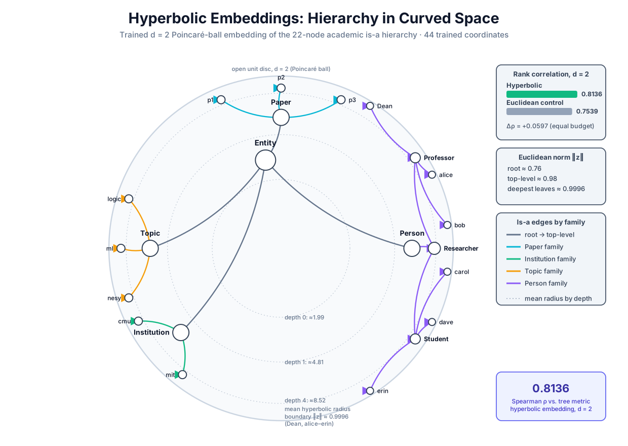The committed d = 2 Poincaré embedding of the academic is-a tree: the root near the center, each generation pushed outward, every family in its own angular sector, and the ball beating the flat plane on rank correlation with the tree metric at the same 44-number budget. Original diagram by the authors, created with AI assistance.

Why two dimensions is the point, not a toy

Choosing $d = 2$ was pedagogically motivated: the trained coordinates are the chapter's figure, nothing projected away, every claim about radii and sectors checkable against the printed coordinate list. But the choice also reflects the field's central empirical finding, which is that hyperbolic embeddings do their best work precisely when dimension is scarce. The original Poincaré-embedding experiments reconstructed the WordNet noun hierarchy, over eighty thousand nodes, with embeddings of dimension five to ten that matched or beat Euclidean embeddings of dimension two hundred [2]; the representation-tradeoffs analysis quantifies why, flat space spending dimensions or distortion on a tree while hyperbolic space spends neither [1]. The result carries to knowledge graphs at large: hyperbolic KG embeddings with relation-specific rotations match state-of-the-art Euclidean models while using an order of magnitude fewer dimensions on hierarchy-rich benchmarks such as WN18RR [3]. The lesson generalizes the counting argument: parameters are a budget, geometry sets the exchange rate, and when the data is tree-shaped, curvature buys what dimensions otherwise would. One caveat keeps the claim honest: curvature is a prior, paying off exactly insofar as the data matches its growth pattern. The academic KG's non-hierarchical relations (citation, authorship, affiliation) carry cycles and cross-links a tree geometry has no special room for, which is one reason practical systems learn the curvature per relation rather than fixing one curved space for everything [3].

Entailment cones: Part II's regions, bent into the ball

The distance-only objective above recovered the hierarchy's levels, but it represents each node as a point, so it still cannot assert subsumption; Part II argued that entailment needs regions with containment. The two ideas compose. Hyperbolic entailment cones carve out, at each point $\mathbf{x}$ of the Poincaré ball outside a small ball around the origin (the construction excludes an $\varepsilon$-neighborhood of the center, where no valid cone aperture exists), a cone $\mathfrak{S}_{\mathbf{x}}$ opening away from the origin, with an aperture that narrows as $\lVert\mathbf{x}\rVert$ grows: widest for general concepts just outside that excluded core, vanishing toward the rim. The concept at $\mathbf{x}$ entails everything embedded inside its cone, and the construction makes membership transitive: if $\mathbf{y} \in \mathfrak{S}_{\mathbf{x}}$ then $\mathfrak{S}_{\mathbf{y}} \subseteq \mathfrak{S}_{\mathbf{x}}$, the geometric image of the fact that subsumption chains (and that nesting is exactly why deeper points must carry narrower cones) [4]. Where Part II's flat cones and boxes fought for volume (a general concept in flat space must be geometrically enormous to contain all its descendants), a wide cone anchored near the origin fans out into the exponential room toward the rim, which is what gives it space for every descendant: Person's cone can hold Researcher's narrower cone, which holds Professor's, which holds alice, without any of them starving for space; training minimizes a margin loss on a cone-membership energy, with substantial reported gains over both distance embeddings and flat order embeddings on WordNet [4]. We do not reimplement cones here; the point is the composition itself, regions for logic and curvature for hierarchy in one geometry, the same design space that EL Embeddings through TransBox and mOWL explored in flat space, reopened in curved space.

The unsolved part

Within its own frame the chapter leaves an honest crack visible: the run's distortion row shows that the ball's win is about ordering, not proportional faithfulness, and near the rim the model runs into arithmetic itself. At the projection shell $1-10^{-5}$, the difference $1-\lVert\mathbf{x}\rVert^2$ that every formula divides by is around $2\times10^{-5}$; the deepest committed points sit at norm $0.9999$, and each further generation of a bigger tree would need another factor-of-$e$ sliver of the remaining space. Representing depth-$k$ nodes faithfully takes on the order of $k$ bits of the gap to the boundary, so float precision, not data, becomes the binding constraint on deep hierarchies [1]; an active line of later work has proposed fixes ranging from alternative charts of hyperbolic space to multi-precision arithmetic.

But the larger unsolved part frames the whole of Parts I–III. Every model in these eleven chapters, TransE's translations, the boxes and balls and cones, and now the curved ball, shares one silent design decision: the embedding of each entity or concept is a free row in a lookup table, adjusted by gradients but structurally independent of every other row. The graph's wiring enters only through the loss, one edge at a time; no model ever computes a node's representation from its neighborhood. That has a concrete cost the running example makes plain: a new node (a new student, a freshly published paper) has no row, so nothing can be predicted about it without retraining, and two nodes with identical surroundings learn unrelated vectors unless the loss happens to push them together. The meaning of a node in a graph lives substantially in its wiring, and what is missing is an encoder that consumes the wiring itself, computing each node's vector from its neighbors' vectors, recursively, so that structure determines representation rather than merely constraining it. Building that encoder, and discovering the precise logical ceiling on what it can distinguish, is Part IV.

Why it matters

For the neuro-symbolic program, this chapter delivers two load-bearing facts. First, geometry is a modeling choice with a logic-shaped payoff: the is-a backbone of every ontology this series cares about (the academic TBox, SNOMED CT, the Gene Ontology, WordNet) is tree-like, the counting argument proves flat space must pay for that shape in dimension or distortion, and curved space pays nothing. When Volume 4 makes logical structure differentiable, a space whose distances already respect the hierarchy hands the learner the ontology's skeleton for free, at a budget small enough to inspect. Second, the committed run is a miniature of the soundness probing this series keeps returning to: a distance-only objective never told about depth or subsumption produced radii that order the generations exactly, and where the geometry only partially honors the logic (rank order yes, proportional distances no), the asserts say so precisely. Reading logical structure off learned geometry, and knowing how far to trust the reading, is the discipline the integration volume depends on.

Key terms

• b-ary tree / branching factor: a tree whose internal nodes each have $b$ children, so depth $k$ holds $b^k$ nodes; exponential growth flat space cannot match.
• Packing bound: the volume argument showing at most $(2k+1)^d$ points with pairwise distance at least $1$ fit in a radius-$k$ Euclidean ball; polynomial capacity against the tree's exponential demand.
• Distortion: the disagreement between graph distance and embedding distance; here scale-fitted as the mean of $\lvert d_{\text{emb}}/(s\,d_{\text{graph}})-1\rvert$ over all $231$ pairs.
• Poincaré ball: the open unit ball $\lVert\mathbf{x}\rVert \lt 1$ with the conformal metric factor $\lambda_{\mathbf{x}} = 2/(1-\lVert\mathbf{x}\rVert^2)$; room grows exponentially with radius and the rim is infinitely far away.
• Geodesic: the shortest path between two points as the space's own metric measures length; in the ball, an arc bowing toward the center.
• Poincaré distance: $d(\mathbf{u},\mathbf{v}) = \operatorname{arcosh}\big(1+2\lVert\mathbf{u}-\mathbf{v}\rVert^2/((1-\lVert\mathbf{u}\rVert^2)(1-\lVert\mathbf{v}\rVert^2))\big)$; radially, $d(\mathbf{0},\mathbf{x}) = 2\operatorname{artanh}\lVert\mathbf{x}\rVert$.
• Riemannian gradient / Riemannian SGD: the steepest-descent vector under the space's metric, here the Euclidean gradient rescaled by $(1-\lVert\boldsymbol{\theta}\rVert^2)^2/4$, followed by projection back into the ball.
• Burn-in: the schedule's first epochs at a reduced learning rate, letting the near-origin initialization organize before full-strength updates.
• Spearman rank correlation: the Pearson correlation of rank vectors, tie-aware; whether the embedding orders the $231$ pairs as the tree does.
• Hyperbolic entailment cone: a region of the ball opening away from the origin whose transitive containment encodes subsumption, uniting Part II's regions with this chapter's curvature.

Where this leads

Part III closes with the hierarchy literally visible in the geometry: radius as depth, sectors as families, subsumption as containment-in-curvature. What no model so far has done is look at the graph while encoding: every vector in Parts I–III is a trained table entry, and the wiring only ever spoke through the loss. The next chapter, Message Passing, inverts that design. Each node's representation will be computed, layer by layer, from the representations of its neighbors, so that the graph's structure becomes the network's computation graph; the same academic KG will flow through the aggregate-and-update equations of the graph neural network (GNN) blueprint, and a new question will immediately arise, one with a precisely logical answer: what can a network that only sees its neighbors ever learn to distinguish?

---

Companion code: examples/neural/hyperbolic.py builds the 22-node hierarchy from Volume 2's concept spine plus kg.TYPE_OF, implements the Poincaré distance, its hand-derived gradients, Riemannian SGD with the ball projection, and the identically-configured Euclidean control, then evaluates both against the BFS tree metric. Run python3 examples/neural/hyperbolic.py to reproduce every number in this chapter; its asserts guard the Spearman win, the strictly increasing norm-vs-depth table, and that every trained point stays inside the open ball.