The Expressiveness Ceiling: 1-WL, C², and Graded Modal Logic

📍 Where we are: Part IV · Graph Neural Networks and Their Ceiling — Chapter 14. Relational GNNs gave every relation its own weight matrix and won the ablation four out of four; this chapter asks what any message-passing network, typed or untyped, deep or shallow, can distinguish at all, and answers exactly.

The last two chapters built increasingly capable machines on one skeleton: a node updates its state from its own current state and the states of its neighbors, layer after layer. This chapter stops tuning that skeleton and proves its boundary. A classical combinatorial procedure, one-dimensional Weisfeiler-Leman color refinement (1-WL, also called color refinement), iteratively colors the nodes of a graph, and the theorem at the heart of Part IV is that no message-passing network, however wide, deep, or cleverly parameterized, can distinguish two nodes or two graphs that 1-WL colors identically [1][2]. The boundary is not folklore; it is low enough to hit with a six-node graph, and the companion file examples/neural/wl.py hits it. Better still, the boundary is a logic: nodes that 1-WL cannot separate are exactly the nodes that agree on every formula of the two-variable counting logic C² [3], and the logical (first-order-expressible) node classifiers a plain message-passing network can express are exactly those of graded modal logic [4]. For a reader coming from Volume 2, that last fact is the payoff of the chapter: it converts "can a GNN check this ontology condition?" from a matter of opinion into a lookup.

The simple version

Imagine a census of two towns where nobody has a name. Each person starts with the same blank badge. Every round, each person fills out one card: "my current badge, plus a tally of my neighbors' current badges," and the census office prints new badges so that identical cards get identical badges and different cards get different ones. Rounds repeat until the badges stop changing. Now the punchline: one town's friendships form two separate three-person triangles, the other town's form one big six-person ring. These towns are genuinely different, but in both, every single person has exactly two friends, so every card reads "blank badge, two blank-badge friends" forever, and the census ends with everyone identical in both towns. Any question you answer by reading badges gets the same answer in both towns. Message-passing networks are badge-readers: a node only ever learns what its neighbors' current summaries say, never who its neighbors actually are, so anything the census cannot see, no GNN can see either.

What this chapter covers

• The refinement algorithm, decoded then quoted: colors start uniform; each round hashes (own color, sorted multiset of neighbor colors); a round that splits nothing certifies the fixpoint. The real loop from wl.py.
• The academic graph, fully resolved: the committed per-round color counts 1 → 5 → 12 → 13, which entities stay merged at each round and why, ending with every entity structurally named.
• The classic failure, run not narrated: two disjoint triangles versus one hexagon: provably non-isomorphic (2 triangles versus 0), yet the committed histograms are identical, so no message-passing function separates them.
• Why the ceiling holds: an induction over layers: a layer sees exactly what a 1-WL round hashes; where injectivity of aggregation enters, and what it buys.
• The injectivity frontier inside the ceiling: sum can represent a neighbor multiset injectively, mean and max cannot; the committed sum/mean/max table on four witness multisets, the base-expansion construction, and the GIN theorem.
• The logic of the ceiling: 1-WL indistinguishability coincides with agreement on all of C²; the first-order-expressible classifiers of plain aggregate-combine GNNs are exactly graded modal logic; the committed class-constancy check.
• Volume 2 read through the ceiling: ∃r.C and ≥n r.C live below it; role composition needs a third variable and lives above it, with a concrete witness pair sinking the grandAdvisor chain for encode-then-score models.
• Ways over the ceiling, priced honestly: k-WL networks, unique identifiers, and subgraph or positional encodings, each with its cost.

The refinement algorithm: hash your neighborhood until nothing splits

First the objects, in plain language. A coloring of a graph assigns each node a label from some finite set; we will use small integers and write $c_k(v)$ for the color that node $v$ carries after round $k$, so the subscript $k$ counts refinement rounds and $v$ ranges over nodes. The neighborhood $N(v)$ is the set of nodes adjacent to $v$. A multiset is a collection in which the same element may appear several times and only the counts matter, not any order; we write it with doubled braces, $\{\!\{ 1, 1, 2 \}\!\}$, to distinguish it from an ordinary set. Finally, a function is injective if distinct inputs always produce distinct outputs, so nothing gets merged.

1-WL color refinement is then three sentences. Start with every node the same color: $c_0(v) = 0$ for all $v$. In each round, every node computes its signature, the pair of its own current color and the multiset of its neighbors' current colors, and an injective relabeling turns each distinct signature into a fresh color:

$$c_{k+1}(v) \;=\; \operatorname{relabel}\Big( c_k(v),\; \{\!\{\, c_k(u) : u \in N(v) \,\}\!\} \Big).$$

Stop when a round changes nothing, meaning the partition of nodes into color classes after the round is the same as before it. Two observations make the loop well behaved. Refinement only ever splits classes, never merges them: nodes colored differently at round $k$ have signatures differing in the first component at round $k+1$, so they stay different. And since a graph with $n$ nodes admits at most $n$ classes, the loop stops within $n$ rounds; a round that splits nothing certifies that no later round could split anything, because every future signature is computed from an unchanged partition.

Here is the loop exactly as committed, wl.py lines 104–119. The textbook "injective hash" is implemented as the rank of each signature among the round's sorted distinct signatures, which is injective by construction and gives canonical small integers:

    colour: dict[str, int] = {v: 0 for v in g}       # round 0: everyone colour 0
    history: list[dict[str, int]] = [colour]
    while True:
        # The 1-WL update:  c_{k+1}(v) = relabel( c_k(v), {{ c_k(u) : u ∈ N(v) }} )
        # where {{...}} is the MULTISET of neighbour colours, here represented
        # as a sorted tuple.  ``relabel`` in the textbook formulation is an
        # injective hash; we use the rank of the signature among the round's
        # distinct signatures in sorted order — injective by construction, so
        # no hash collisions, and canonical small ints each round.
        sig = {v: (colour[v], tuple(sorted(colour[u] for u in g[v]))) for v in g}
        canon = {s: i for i, s in enumerate(sorted(set(sig.values())))}
        new = {v: canon[sig[v]] for v in g}
        history.append(new)
        if _partition(new) == _partition(colour):    # nothing split: fixpoint
            return history, len(history) - 1
        colour = new

Note what this procedure is allowed to see. It reads the graph as undirected and unlabeled: relation types and edge directions are exactly the information color refinement throws away, and the companion file is explicit about this when it builds the 1-WL view of the running example (wl.py lines 66–74):

def academic_graph() -> Graph:
    """The running example as 1-WL sees it: the 18 triples become 18 undirected,
    unlabelled edges over the 13 entities (relation types and directions are
    exactly the information colour refinement throws away)."""
    adj: dict[str, set[str]] = defaultdict(set)
    for h, _r, t in kg.TRIPLES:
        adj[h].add(t)
        adj[t].add(h)
    return {v: tuple(sorted(adj[v])) for v in sorted(adj)}

This is the honest baseline for the untyped GCN (graph convolutional network) of Message Passing. Typed message passing, as in the previous chapter's R-GCN (relational graph convolutional network), corresponds to running 1-WL on the labeled graph, where each round's signature carries one neighbor multiset per relation; that variant refines faster, and the theory below holds verbatim for it [2][5].

Round by round on the academic graph

Run python3 wl.py and exhibit 2 traces refinement on the 13 entities and 18 undirected edges of the academic world. This is the committed output:

exhibit 2 — 1-WL on the academic graph (13 nodes, 18 edges)
  colours per round: 1 -> 5 -> 12 -> 13 -> 13 (stable: round 4 reproduces round 3)
  round 1 non-singleton classes: {logic, ml, nesy}  {erin, mit}  {alice, cmu, dave, p3}  {carol, p1, p2}
  round 2 non-singleton classes: {logic, nesy}
  round 1 is exactly the degree partition; round 2 still cannot
  split logic from nesy (each has one neighbour, a degree-4 paper);
  round 3 splits them because p1 and p2 got different colours.
  fixpoint: 13 colours for 13 nodes — entities sharing a colour: none
  (the discrete partition: 1-WL names every individual here,
   in contrast with exhibit 1)

Decode the trace. Round 0 is the uniform start, one color. In round 1 every node's signature is $(0, \{\!\{0, \ldots, 0\}\!\})$ with as many zeros as it has neighbors, so the only distinguishing feature is how many neighbors: round 1 is exactly the partition by degree, the number of edges at a node. The academic graph has five distinct degrees, hence five classes:

degree	entities in the class	who they are
1	logic, ml, nesy	the three topics, each attached to one paper
2	erin, mit	a student with two ties; an institution with two members
3	alice, cmu, dave, p3	a professor, an institution, a student, a paper
4	carol, p1, p2	a student and two well-connected papers
5	bob	the hub: adviser, author, employee at once

The degree-3 row is worth staring at: four entities of four different ontological types share a color after one round, precisely the situation that motivated relation typing in the previous chapter. Round 2 splits almost everything, 5 classes becoming 12, because second-round signatures see the degrees of the neighbors. The one class it cannot split is $\{$logic, nesy$\}$: each is a degree-1 topic whose single neighbor is a degree-4 paper (p1 for logic, p2 for nesy), so both present the same signature to round 2 (built from round-1 colors): "degree-1 node attached to a degree-4 node." Round 3 finishes the job, but only because the papers separated in round 2: p1's neighbors are alice, bob, logic, p2 while p2's are carol, nesy, p1, p3, neighborhoods with different degree profiles, so $c_2(\mathrm{p1}) \neq c_2(\mathrm{p2})$, and in round 3 the topics inherit the difference. Information propagates one hop per round, so a node is distinguished in round $k+1$ by structure $k+1$ hops away.

The fixpoint is the discrete partition: 13 colors for 13 nodes, no two entities structurally indistinguishable, reached at round 3 and certified in round 4 (round 4 reproduces round 3; academic_rounds=4 in the summary line). On this graph, 1-WL names every individual by structure alone. Hold that thought, because on the next graph it can name nothing at all.

The failure exhibit: two triangles versus a hexagon

Exhibit 1 builds two graphs with six nodes each, using the cycle constructor (wl.py lines 48–53): $G_1$ is the disjoint union of two 3-cycles ($2 \times C_3$, nodes x0 x1 x2 y0 y1 y2), and $G_2$ is the single 6-cycle ($C_6$, nodes z0 through z5). These graphs are provably non-isomorphic, meaning no relabeling of nodes turns one into the other: the number of triangles (3-cliques) is a subgraph invariant, and the committed counts are 2 for $G_1$ and 0 for $G_2$. Yet every node in both graphs is 2-regular, having exactly two neighbors. Run 1-WL on the disjoint union of both graphs (the standard way to compare two graphs with shared, comparable colors) and this happens:

exhibit 1 — the classic failure: two triangles vs one hexagon
  G1 = C3 + C3 (nodes x0 x1 x2 y0 y1 y2)   triangles: 2
  G2 = C6      (nodes z0 z1 z2 z3 z4 z5)   triangles: 0
  triangle counts differ -> the graphs are NOT isomorphic
  1-WL on the disjoint union (12 nodes, colours comparable):
    round 0: 1 colour (uniform start)
    round 1: every node has signature (0, (0, 0)) — all 2-regular —
             nothing splits; stable after 1 round
  histogram(G1) = {0: 6}    histogram(G2) = {0: 6}    identical = True
  1-WL returns 'possibly isomorphic' for provably different graphs,
  so no message-passing GNN can embed G1 and G2 differently.

The mechanism is visible in the signature: all twelve nodes carry color 0, all have exactly two color-0 neighbors, so all twelve signatures are $(0, \{\!\{0, 0\}\!\})$, nothing splits, and the uniform coloring is already the fixpoint after a single certifying round. The stable color histogram, the map from each color to how many nodes carry it, is $\{ 0 \mapsto 6 \}$ for both graphs: identical. 1-WL's verdict on the pair is "possibly isomorphic," and that verdict is wrong, since the triangle counts already proved otherwise. The companion file pins each of these claims with an assertion (wl.py lines 273–275):

    assert tri1 == 2 and tri2 == 0, "triangle counts must prove non-isomorphism"
    assert hist_g1 == hist_g2, "1-WL must FAIL to separate 2xC3 from C6"
    assert rounds1 == rounds2 == union_rounds == 1, "2-regular graphs are stable at once"

State plainly what follows, because it is the strongest sentence in this chapter. Once the ceiling theorem of the next section is in place, this exhibit implies: any function computed by message passing, any GCN, any R-GCN, any architecture that updates nodes from neighbor multisets and reads out a permutation-invariant summary, takes the same value on $G_1$ and $G_2$. In particular, no message-passing GNN can compute, or even approximate on both inputs at once, the function "how many triangles does this graph contain," or the property "some node lies on a triangle," because those functions differ on a pair the network provably cannot tell apart [1][2]. Triangle counting is not hard for message passing; it is beyond it.

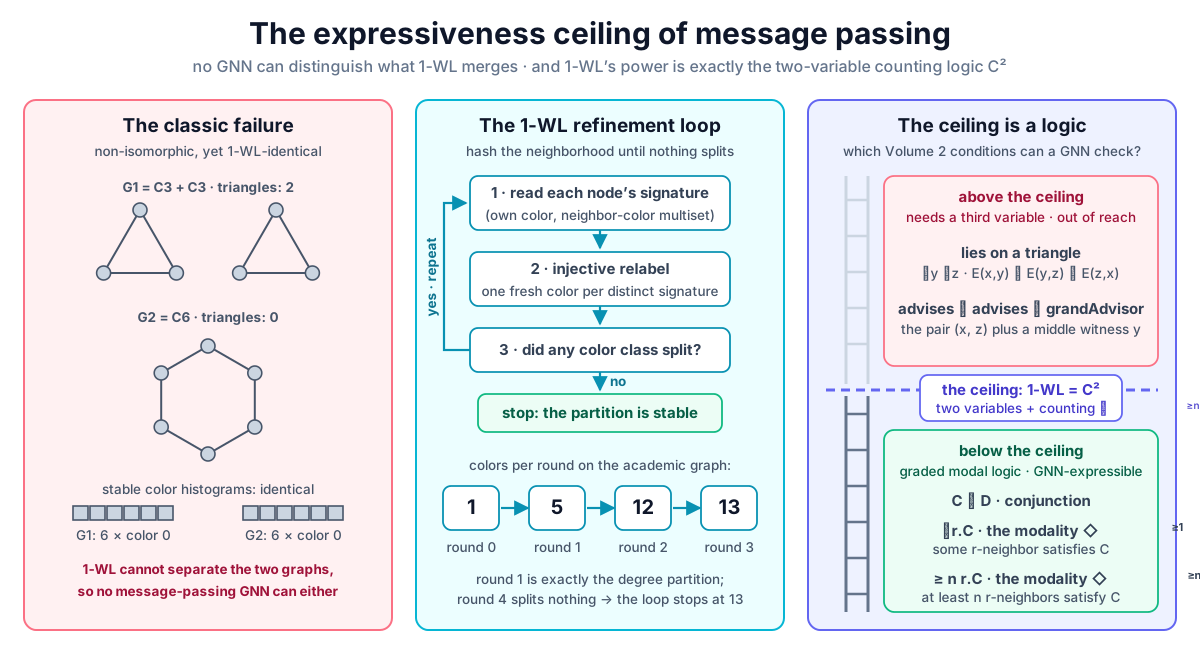The ceiling in one picture: 1-WL refinement (center) resolves the academic graph completely but cannot split two triangles from a hexagon (left), and the counting logic C² (right) says exactly which conditions live below the line message passing cannot cross. Original diagram by the authors, created with AI assistance.

Why the ceiling holds

The theorem deserves a real argument, not intimidation, and the argument is a short induction. Fix the notation of the last two chapters: a message-passing network computes, for each node $v$ and each layer $k$, a hidden state $\mathbf{h}_v^{(k)} \in \mathbb{R}^d$ (a vector of $d$ real numbers, $d$ being the layer width), by the generic two-step update

$$\mathbf{h}_v^{(k)} \;=\; \mathrm{COMBINE}^{(k)}\Big( \mathbf{h}_v^{(k-1)},\; \mathrm{AGGREGATE}^{(k)}\big( \{\!\{\, \mathbf{h}_u^{(k-1)} : u \in N(v) \,\}\!\} \big) \Big),$$

where AGGREGATE maps a multiset of neighbor states to a summary (the degree-normalized average in the GCN, which [1] analyzes in its element-wise mean-pooling form; the R-GCN's per-relation normalized sum is the labeled-variant instance, one aggregated multiset per relation) and COMBINE fuses that summary with the node's own state. The functions can be anything at all, linear maps, multilayer perceptrons, learned or hand-set; the only structural commitment is that layer $k$'s input for node $v$ is exactly the pair (own previous state, multiset of neighbors' previous states). That pair is also exactly what a 1-WL round hashes. The theorem turns this coincidence into a bound [1][2].

Theorem (the ceiling). Let all nodes start with identical initial features, $\mathbf{h}_v^{(0)} = \mathbf{h}_w^{(0)}$ for all $v, w$, matching 1-WL's uniform start. Then for every layer count $k$ and all nodes $u, v$ (in one graph or across two graphs refined jointly): if $c_k(u) = c_k(v)$ then $\mathbf{h}_u^{(k)} = \mathbf{h}_v^{(k)}$. Equal 1-WL colors force equal hidden states, so a GNN can only separate what 1-WL separates.

Proof, by induction on $k$. The base case $k = 0$ is the hypothesis: all initial colors are equal and all initial features are equal, so the implication holds immediately. For the inductive step, assume the claim at layer $k$ and suppose $c_{k+1}(u) = c_{k+1}(v)$. The relabeling in the 1-WL update is injective, and an injective function returns equal outputs only on equal inputs, so the two signatures must be equal as pairs:

$$c_k(u) = c_k(v) \qquad\text{and}\qquad \{\!\{\, c_k(w) : w \in N(u) \,\}\!\} \;=\; \{\!\{\, c_k(w') : w' \in N(v) \,\}\!\}.$$

The first equality feeds the induction hypothesis directly: $\mathbf{h}_u^{(k)} = \mathbf{h}_v^{(k)}$. The second says the two neighbor color multisets agree, and two finite multisets are equal exactly when there is a bijection (a one-to-one, onto matching) $\pi : N(u) \to N(v)$ with $c_k(w) = c_k(\pi(w))$ for every neighbor $w$ of $u$; in particular $u$ and $v$ have the same number of neighbors. Apply the induction hypothesis to each matched pair: $c_k(w) = c_k(\pi(w))$ gives $\mathbf{h}_w^{(k)} = \mathbf{h}_{\pi(w)}^{(k)}$. A bijection that matches equal elements to equal elements means the state multisets are equal too:

$$\{\!\{\, \mathbf{h}_w^{(k)} : w \in N(u) \,\}\!\} \;=\; \{\!\{\, \mathbf{h}_{w'}^{(k)} : w' \in N(v) \,\}\!\}.$$

Now both inputs to layer $k+1$ agree for $u$ and $v$: the own states are equal, and the neighbor multisets are equal. AGGREGATE and COMBINE are functions, and a function applied to equal inputs returns equal outputs, whatever the function is. Therefore $\mathbf{h}_u^{(k+1)} = \mathbf{h}_v^{(k+1)}$, which completes the induction. $\blacksquare$

Two remarks put the proof to work. First, the graph-level consequence claimed in the failure exhibit follows in one line: a graph-level prediction is a readout applied to the multiset of final node states, and on $2 \times C_3$ and $C_6$ those multisets are identical (six copies of the same vector on each side), so every readout agrees. Second, notice where the proof does not use injectivity: AGGREGATE and COMBINE may be arbitrary, and the bound still holds. Injectivity matters for the converse, whether a GNN climbs all the way up to the ceiling rather than sitting below it. If some layer's aggregation merges two neighbor multisets that 1-WL would tell apart, the network is strictly weaker than 1-WL; if every layer's (state, multiset) map is injective, a symmetric induction shows equal hidden states force equal colors, and the network matches 1-WL exactly [1]. So the practical question inside the ceiling becomes: which aggregators are injective on multisets?

Sum, mean, max: the injectivity frontier

Exhibit 3 answers with four witness multisets, arranged in two pairs so that each aggregator's blind spot is isolated (wl.py lines 214–217):

    m1 = np.array([1.0, 1.0, 2.0, 2.0])   # M1 = {{1,1,2,2}}  (= M2 duplicated)
    m2 = np.array([1.0, 2.0])             # M2 = {{1,2}}
    m3 = np.array([1.0, 1.0, 2.0])        # M3 = {{1,1,2}}  same set {1,2} as M4,
    m4 = np.array([1.0, 2.0, 2.0])        # M4 = {{1,2,2}}  different multiplicities

The committed run aggregates each pair three ways:

exhibit 3 — aggregators on neighbour multisets (the GIN argument)
  pair      A            B          mean(A) mean(B)  max(A) max(B)  sum(A) sum(B)  separated by
  M1 vs M2  {1,1,2,2}    {1,2}       1.5000  1.5000     2.0    2.0     6.0    3.0  sum
  M3 vs M4  {1,1,2}      {1,2,2}     1.3333  1.6667     2.0    2.0     4.0    5.0  sum, mean
  sum separates both pairs; mean misses the k-fold copy (M1 = 2·M2);
  max misses multiplicities (M3, M4 share the set {1, 2}).

pair	multisets	mean	max	sum
$M_1$ vs $M_2$	$\{\!\{1,1,2,2\}\!\}$ vs $\{\!\{1,2\}\!\}$	$1.5 = 1.5$ ✗	$2.0 = 2.0$ ✗	$6.0 \neq 3.0$ ✓
$M_3$ vs $M_4$	$\{\!\{1,1,2\}\!\}$ vs $\{\!\{1,2,2\}\!\}$	$1.3333 \neq 1.6667$ ✓	$2.0 = 2.0$ ✗	$4.0 \neq 5.0$ ✓

Each failure has a one-line derivation, not just a witness. Mean sees only the distribution. Write $|M|$ for the size of a multiset $M$ and let $kM$ be its $k$-fold copy, every multiplicity multiplied by $k$. Then the sum scales as $\operatorname{sum}(kM) = k \cdot \operatorname{sum}(M)$ and the size as $|kM| = k\,|M|$, so

$$\operatorname{mean}(kM) \;=\; \frac{\operatorname{sum}(kM)}{|kM|} \;=\; \frac{k \cdot \operatorname{sum}(M)}{k\,|M|} \;=\; \operatorname{mean}(M),$$

and $M_1 = 2 M_2$ exactly, so no mean-aggregating layer can distinguish a neighborhood from its doubled copy. Max sees only the underlying set. The maximum of a multiset depends only on which elements appear, never on how often, and $M_3, M_4$ share the set $\{1, 2\}$, so max ties (their means differ, $4/3$ versus $5/3$, which is why the second row's mean check passes). Sum sees everything, and this is a theorem, not luck, provided the elements come from a countable domain (one whose members can be listed $x_1, x_2, x_3, \ldots$, which covers every domain a digital computer can represent). Here is the construction with every step shown [1]. Suppose all neighborhoods have size at most $N$. Encode the $i$-th element of the domain as the number $f(x_i) = (N+1)^{-i}$. A multiset $M$ with multiplicities $m_1, m_2, m_3, \ldots$ (element $x_i$ appearing $m_i$ times, finitely many nonzero, each $m_i \le N$) then sums to

$$\sum_{x \in M} f(x) \;=\; \sum_{i \ge 1} m_i\, (N+1)^{-i},$$

which is precisely the number whose base-$(N+1)$ expansion has digit $m_i$ in position $i$. To see the sum determines every $m_i$, suppose two multisets $M \neq M'$ with digit sequences $m_i$ and $m_i'$ had equal sums, and let $j$ be the smallest position where the digits differ. The difference of the sums is

$$\big(m_j - m_j'\big)(N+1)^{-j} \;+\; \sum_{i > j} \big(m_i - m_i'\big)(N+1)^{-i}.$$

The first term has absolute value at least $(N+1)^{-j}$, because $m_j \neq m_j'$ are integers so they differ by at least 1. The tail is bounded by the geometric series in which every digit gap takes its largest possible value $N$:

$$\Big|\sum_{i > j} (m_i - m_i')(N+1)^{-i}\Big| \;\le\; \sum_{i > j} N (N+1)^{-i} \;=\; N \cdot \frac{(N+1)^{-(j+1)}}{1 - \frac{1}{N+1}} \;=\; N \cdot \frac{(N+1)^{-(j+1)} (N+1)}{N} \;=\; (N+1)^{-j},$$

with equality only if infinitely many digit gaps equal $N$, which finite multisets cannot achieve; the tail is therefore strictly smaller than $(N+1)^{-j}$ and cannot cancel the first term. The difference is nonzero, the sums differ, and $f$ followed by summation is injective on all multisets of size at most $N$. Sum aggregation, unlike mean and max, can carry a full, lossless fingerprint of the neighborhood.

The Graph Isomorphism Network (GIN) is the architecture built on exactly this observation [1]. Its layer is

$$\mathbf{h}_v^{(k)} \;=\; \mathrm{MLP}^{(k)}\Big( \big(1 + \varepsilon^{(k)}\big)\, \mathbf{h}_v^{(k-1)} \;+\; \sum_{u \in N(v)} \mathbf{h}_u^{(k-1)} \Big),$$

where the scalar $\varepsilon^{(k)}$ keeps the node's own state from being absorbed into the neighbor sum. For a suitable choice of $\varepsilon^{(k)}$ (any irrational value suffices when the features range over a countable domain [1]), the layer is injective on the pair (own state, neighbor multiset) and not just on the multiset; an arbitrary value, such as the $\varepsilon = 0$ of the common GIN-0 variant, carries no such guarantee. The multilayer perceptron supplies the arbitrary function composed with the injective encoding. The resulting theorem is the exact frontier inside the ceiling: a message-passing GNN with injective aggregation and combination distinguishes everything 1-WL distinguishes and, by the ceiling theorem, nothing more, so GIN is a maximally powerful message-passing architecture [1][2]. Mean-aggregating architectures, including the GCN in the mean-pooling form that [1] analyzes, sit strictly below the frontier (they cannot even tell a neighborhood from its double); nothing sits above it while remaining message passing. The committed assertions record the frontier numerically (wl.py lines 276–279), and the summary line reports sum_separates=2/2 mean_separates=1/2 max_separates=0/2.

The logic of the ceiling: C² and graded modal logic

So far the ceiling is combinatorial: "whatever 1-WL cannot split." The most useful theorem in this chapter converts it into logic, and it predates GNNs by decades [3][6]. Define C² as first-order logic restricted to exactly two variable symbols, $x$ and $y$, reusable by nested quantifiers, and extended with counting quantifiers $\exists^{\ge n}$, where $\exists^{\ge n} y\, \varphi(x, y)$ reads "there exist at least $n$ distinct $y$ making $\varphi$ true." Write $E(x, y)$ for the edge relation, read "there is an edge between $x$ and $y$," and $\wedge$ for conjunction, read "and." Reuse is the subtle power: the formula

$$\varphi(x) \;=\; \exists y \Big( E(x,y) \;\wedge\; \exists x \big( E(y,x) \big) \Big)$$

says "$x$ has a neighbor that has a neighbor," reusing $x$ inside the inner quantifier for a new role, and it is a legal C² formula: two hops with two variables. The characterization theorem states that two nodes receive the same stable 1-WL color if and only if they satisfy exactly the same C² formulas in one free variable, and two graphs are 1-WL-indistinguishable if and only if they satisfy the same C² sentences (formulas with no free variable) [3][6]; more generally, the $k$-dimensional generalization of WL corresponds in the same way to the logic with $k+1$ variables, $\mathrm{C}^{k+1}$ [3][5]. Composed with the ceiling theorem, this hands the neuro-symbolic reader a precise slogan: a message-passing GNN can separate two nodes only if some C² formula separates them. The ceiling is not an architecture quirk; it is the expressive reach of a two-variable counting logic.

A corollary is checkable by program: every C²-expressible node property must be constant on every stable color class, since same color means same C² properties. Exhibit 4 checks it with the graded formula $\varphi(x) = \exists^{\ge 2} y\, E(x,y)$, "x has at least 2 neighbors" (wl.py lines 257–261, using constant_on_classes from lines 137–144):

    def phi(graph: Graph) -> Callable[[str], bool]:
        return lambda v: len(graph[v]) >= 2

    c2_academic = constant_on_classes(stable_acad, phi(acad))
    c2_union = constant_on_classes(stable_union, phi(union))

exhibit 4 — counting logic: the ceiling is exactly C²
  theorem: same stable 1-WL colour  <=>  same C² properties
  witness φ(x) = 'x has at least 2 neighbours'  (∃^{≥2} y. E(x,y))
  academic graph: φ constant on all 13 stable classes -> True
  triangles-vs-hexagon union: φ constant on the single 12-node class -> True

On the academic graph the check is easy (13 singleton classes can never be split by anything), but on the triangles-versus-hexagon union it bites: the single 12-node class must give one answer, and it does, since all twelve nodes are 2-regular and $\varphi$ holds of every one.

For node classifiers, the fragment can be pinned down even more tightly [4]. Graded modal logic is the local fragment of C²: formulas are built from node labels and Boolean connectives plus the graded modality $\Diamond^{\ge n} \varphi$, "at least $n$ of my neighbors satisfy $\varphi$," so every quantifier is guarded by the edge relation and evaluation only looks outward from the node through edges. The correspondence theorem says a logical node classifier is expressible by a plain aggregate-combine GNN, the Part IV blueprint, exactly when it is definable in graded modal logic; extending the architecture with a global readout in every layer (the ACR-GNN, for aggregate-combine-readout) can express every classifier in the unary fragment of C², picking up non-local conditions such as "the graph somewhere contains an isolated node" that no purely local exchange can reach [4]. (For the readout variant this is a containment, not an equivalence: every unary C² classifier has an ACR-GNN, while the exact logical characterization of ACR-GNNs remains open.) Read the two levels as contracts: the blueprint checks any condition phrased as nested graded modalities over node labels, nothing else; a readout buys the rest of C², but never a third variable.

Volume 2 read through the ceiling

Now hold the C² lens up to the description logic of Volume 2, because the two vocabularies translate almost word for word. A concept membership check "does entity $x$ satisfy concept $C$" is a node property; a role is an edge relation. Three more symbols need decoding before the table: $\top$ is the universal concept, the concept every entity satisfies, so $\exists r.\exists r.\top$ reads "related by $r$ to something that is itself related by $r$ to something"; $\circ$ is role composition, so $r \circ s$ relates $x$ to $z$ whenever an $r$-step from $x$ reaches some $y$ and an $s$-step from $y$ reaches $z$; and $\sqsubseteq$ is subsumption, read "is contained in," so the axiom's left-hand side implies its right-hand side. Line the constructors up:

Volume 2 construct	first-order shape	variables	verdict
conjunction $C \sqcap D$	$C(x) \wedge D(x)$	1	below the ceiling
existential $\exists r.C$	$\exists y\, (r(x,y) \wedge C(y))$	2	below: the modality $\Diamond^{\ge 1}$
number restriction $\ge n\; r.C$	$\exists^{\ge n} y\, (r(x,y) \wedge C(y))$	2	below: the graded modality $\Diamond^{\ge n}$
nested existential $\exists r.\exists r.\top$	$\exists y (r(x,y) \wedge \exists x\, r(y,x))$	2, by reuse	below
"lies on a triangle"	$\exists y \exists z\, (E(x,y) \wedge E(y,z) \wedge E(z,x))$	3	above the ceiling
role chain $\text{advises} \circ \text{advises} \sqsubseteq \text{grandAdvisor}$	$\exists y\, (\text{advises}(x,y) \wedge \text{advises}(y,z))$	3	above the ceiling

The first four rows are good news for graph networks. The workhorse EL constructor $\exists r.C$, "advises some student," is literally the modal operator $\Diamond^{\ge 1}$ applied to a node label, and the qualified number restriction $\ge n\; r.C$ of richer description logics, "advises at least 2 students," is the graded modality $\Diamond^{\ge 2}$ applied to a node label, whose unqualified special case, at least 2 neighbors of any kind, is exactly the property exhibit 4 checks against the stable classes: C²-expressible and GNN-checkable, with the committed run confirming that stable colors respect it. Nested existentials stay below the ceiling too, by the variable-reuse trick shown above. A relational network like the previous chapter's R-GCN can, in principle, learn a classifier for any concept built from these pieces.

The last two rows are the warning. "Lies on a triangle" genuinely requires three simultaneously related objects, and no C² formula expresses it, which is the logical reading of the failure exhibit: $2 \times C_3$ is full of triangle-nodes, $C_6$ has none, and they are C²-equivalent [3][5]. The role-chain row cuts closer to home. Volume 2's completion engine handled the axiom $\text{advises} \circ \text{advises} \sqsubseteq \text{grandAdvisor}$ in a single step: the rule CRχ fused two ledger edges through a shared middle concept. But the defining condition relates a pair $(x, z)$ through a middle witness $y$: three variables live in the formula at once, and no reuse trick eliminates one, because $x$ and $z$ must both remain free while $y$ is quantified. The composed relation is not definable in C².

The failure exhibit's stable coloring turns that non-definability into a concrete impossibility for the standard neural pipeline. Consider any encode-then-score link predictor, the pattern of this whole volume: message passing computes an embedding per node, then a scoring function of the two endpoint embeddings (a TransE distance, a DistMult product, an MLP) decides whether the pair stands in the relation. Run it on the hexagon $C_6$ with uninformative features. By the ceiling theorem every node gets the same embedding, since all six share one stable color. Now compare the pair $(z_0, z_2)$ with the pair $(z_0, z_3)$: $z_0$ and $z_2$ have the common neighbor $z_1$, so a length-2 path connects them and the chain condition holds; $z_0$'s neighbors are $z_1, z_5$ while $z_3$'s are $z_2, z_4$, disjoint sets, so the condition fails. Any score of the form $f(\mathbf{h}_{z_0}, \mathbf{h}_{z_2})$ versus $f(\mathbf{h}_{z_0}, \mathbf{h}_{z_3})$ compares identical arguments and returns identical values; one answer must be wrong. A message-passing GNN cannot, in general, verify the role-chain axiom that Volume 2's completion derived in one rule firing. The honest footnote: the impossibility binds the encode-then-score pattern with structure-only features; predictors that condition on the pair itself, such as the path-based models mentioned at the close of the previous chapter, escape this argument by changing what the network sees.

Ways over the ceiling, priced

The ceiling is a theorem about a computational pattern, so every escape route changes the pattern, and each one pays for its power with something the message-passing blueprint had bought.

Higher-order networks. The $k$-dimensional Weisfeiler-Leman algorithm ($k$-WL) colors ordered $k$-tuples of nodes rather than single nodes, and here the variant names matter, because two different algorithms share the name. The folklore tuple version refines a tuple by recording, for every candidate node $w$, the joint pattern of colors obtained by substituting $w$ into each coordinate in turn, and its discriminating power corresponds exactly to the logic $\mathrm{C}^{k+1}$, strictly increasing with $k$ [3]; the "oblivious" variant more common in the GNN literature aggregates each coordinate's substitutions separately and sits one level lower (its 2-dimensional form has exactly the power of 1-WL). Under the folklore reading, at $k = 2$ triangles become countable and role chains checkable. Neural versions come with the same caveat: the $k$-GNNs of [2] pass messages between $k$-element node sets and provably match a set-based refinement, weaker again than the tuple hierarchy, while tuple-based higher-order architectures do realize the full hierarchy, level by level [5]. The price, for every variant, is the state space. A graph with $n$ nodes has $n^k$ ordered $k$-tuples: our 13-entity toy already has 169 pairs and 2,197 triples, and a graph with a million nodes has $10^{12}$ pairs before a single weight is allocated. The cost is the combinatorics of the object being colored, which is why higher-order networks remain rare outside small-molecule domains.

Unique identifiers and random features. Give every node a distinguishing input feature, a one-hot identity or a random vector, and the ceiling theorem's hypothesis (identical initial features) fails immediately: 1-WL seeded with distinct colors separates everything, and the network can in principle compute any function of the graph. The price is permutation invariance, the guarantee that the output does not depend on the arbitrary order in which nodes happen to be listed. With identities in the input, isomorphic graphs can receive different outputs, what is learned about the node called $z_1$ does not transfer to the structurally identical node called $z_4$, and with random features two runs on the same graph need not even agree. Expressiveness is bought by giving up the symmetry that let a model trained on one part of a graph say anything about another.

Subgraph and positional encodings. The pragmatic middle road precomputes what the network cannot express and appends it to the input features: triangle counts, counts of small subgraphs, distances to anchor nodes, or spectral coordinates from the graph Laplacian's eigenvectors. The augmented model already exceeds plain 1-WL, because 1-WL seeded with triangle counts splits $2 \times C_3$ from $C_6$ in round zero. The price is that the crucial invariant is now chosen, not learned: someone must know in advance that triangles matter, compute them symbolically, and hand them over, and any structure outside the chosen list stays invisible. For a neuro-symbolic reader this road is less a trick than a thesis: the fix for a neural ceiling was a small piece of symbolic preprocessing, Volume 4's pattern in miniature.

The unsolved part

The theorem in this chapter is airtight, and it is also narrower than it looks, in two directions that remain genuinely open. First, the ceiling is a statement about distinguishing, in the worst case, with structure-only inputs; it says nothing about how hard it is to learn the functions inside the ceiling. A GIN can represent the 1-WL fingerprint, but whether gradient descent on a finite sample finds the weights that compute it is a separate question with no comparably clean theorem, and empirically the gap between what an architecture can express and what training reliably reaches is wide. The field has an exact map of expressiveness and only sketches of learnability. Second, and closer to this book's spine: the ceiling binds every architecture that reads fixed wiring, where the graph is given and the computation flows along it. There is another way to use the same vector machinery. Instead of asking "who are my neighbors?" a node can ask "who, among everyone, is relevant to me right now?" and compute the answer from content, building its interaction graph on the fly at every layer. That operation, attention, is not message passing over a fixed graph, so nothing in this chapter bounds it; it has different powers, and different costs, of its own.

Why it matters

This chapter is the closest thing Part IV has to a verdict, and the most directly usable theorem in the volume for a neuro-symbolic engineer. Volume 4 will repeatedly propose neural components that claim to check, enforce, or approximate logical conditions, and the C² correspondence is the lookup table that says in advance which claims are even possible for a message-passing component: graded, local, two-variable conditions, yes; triangles, compositions, chains, no, not without higher-order state, identities, or symbolic features. The role-chain result deserves particular weight. Volume 2's saturated ledger, our gold standard for entailment, contains grandAdvisor edges derived by one rule application; this chapter proved that the dominant neural pattern for knowledge graphs cannot in general reproduce that inference. When a later chapter needs a neural system to respect role composition, it will have to add something, and now we know that necessity is mathematical, not a matter of tuning. Ceilings you can state are ceilings you can design around.

Key terms

• 1-WL color refinement (Weisfeiler-Leman) — the iterative algorithm that recolors each node by an injective hash of its signature, the pair (own color, multiset of neighbor colors), until the partition stabilizes; the exact upper bound on message-passing discrimination.
• Stable partition (fixpoint) — the coloring a refinement round reproduces; refinement only splits classes, so one unproductive round certifies stability forever.
• Multiset — a collection where only element counts matter, written $\{\!\{ \cdot \}\!\}$; the neighbor aggregation input.
• Injective aggregation — a multiset function that never merges distinct multisets; sum admits one over countable domains (the base-$(N+1)$ construction), mean and max do not.
• GIN (Graph Isomorphism Network) — the sum-plus-MLP architecture whose layers are injective on (state, multiset), making it exactly as powerful as 1-WL: the frontier inside the ceiling.
• C² (two-variable counting logic) — first-order logic with two reusable variables and counting quantifiers $\exists^{\ge n}$; same stable 1-WL color coincides with agreement on all C² formulas.
• Graded modal logic — the local fragment of C² built from node labels and modalities $\Diamond^{\ge n}\varphi$ ("at least $n$ neighbors satisfy $\varphi$"); exactly the first-order-expressible node classifiers plain aggregate-combine GNNs can express.
• ACR-GNN — aggregate-combine-readout architecture with a global summary each layer; can express every classifier in the unary fragment of C² (the exact characterization of the architecture itself is open).
• Permutation invariance — independence of the output from node ordering; the property unique identifiers and random features sacrifice for expressiveness.
• k-WL and k-GNNs — the folklore $k$-WL refines ordered $k$-tuples, with power $\mathrm{C}^{k+1}$ and cost $n^k$; the oblivious variant and the set-based $k$-GNNs sit strictly lower in the hierarchy.

Where this leads

Part IV ends at a boundary drawn around a single assumption: the graph is given, and computation flows along its fixed edges. Attention discards the assumption. In an attention layer, every element scores its relevance to every other element from their contents, normalizes the scores, and reads out a weighted blend, in effect constructing a fresh, weighted, complete interaction graph at every layer and every input. That mechanism is the engine of the transformer, and for this book it is more: queries matching keys is the neural echo of a symbolic operation, unification, that Volume 1 built by hand. The next chapter takes attention apart with the same discipline applied here, every matrix decoded, every gradient derived, every number from a committed run, and asks how a mechanism that computes its own wiring relates to the ceiling that fixed wiring could not cross.

---

Companion code: examples/neural/wl.py implements 1-WL color refinement with an injective canonical relabeling, the four exhibits quoted in this chapter (the triangles-versus-hexagon failure, the academic-graph trace, the sum/mean/max multiset table, and the C² class-constancy check), and competency assertions for every claim. Run python3 examples/neural/wl.py to reproduce every number; the module is deterministic by construction, so repeated runs print byte-identical output.