BoxEL and Box²EL: Faithful Ontology Embeddings

📍 Where we are: Part III · Embedding Ontologies — Chapter 9. EL Embeddings trained balls against Volume 2's TBox and audited them with the reasoner's own verdict; this chapter changes exactly one variable, the shape of a concept, and reruns the identical audit with boxes.

The previous chapter ended with a confession built into its own loss function. The ball model could not train a conjunction axiom $A \sqcap B \sqsubseteq C$ (⊓ is concept conjunction, whatever belongs to both $A$ and $B$ ; ⊑ reads "is subsumed by", so the axiom says everything in both $A$ and $B$ is a $C$ ) against the actual intersection of two balls, because that intersection is a lens and a lens is not a ball; it had to substitute a midpoint heuristic and hope the springs settled somewhere reasonable [1]. Boxes versus Balls proved the underlying closure fact with no training in sight. This chapter closes the loop: it takes the same sixteen normal forms, the same recomputed gold standard, the same probe, and trains axis-aligned boxes instead of balls, in the style of BoxEL [2] and its intersection-minded sibling ELBE [3]. One naming precision up front: BoxEL proper scores axioms by box volumes and models a role as a translation plus a per-axis scaling, so the companion's translation-only, corner-hinge core is closest to ELBE's design; this chapter uses the family label for the shape and the citations for the specifics. The payoff is a two-row confusion table in which both rows are recomputed, on identical data against an identical judge, inside a single run.

The simple version

Imagine two city planners handed the same zoning laws. The first planner works only with circular districts. Most laws are easy: "Professor inside Researcher" is one circle drawn inside another. But the law "whatever lies in both the Professor and Researcher districts must lie in the Person district" is about an overlap, and the overlap of two circles is a lens shape the circular toolkit cannot draw; the best available move is a circle around the lens, which quietly annexes land that was never in both districts. The second planner works with rectangular districts, and the overlap of two rectangles is itself a rectangle, its corners read directly off the corners of its parents. Both planners are graded by the same inspector on the same laws. On a small town both earn a perfect score; the difference is that the rectangle planner's perfect score came from measuring, while the circle planner's came from having enough room for luck to work. This chapter is that graded head-to-head, and the rectangles are boxes in eight-dimensional space.

What this chapter covers

A controlled comparison by construction: box_el.py imports the identical data pipeline as the ball model: 14 axioms into 16 normal forms, one role chain skipped out loud, 15 trainable axioms, the 8-pair gold standard recomputed from el_completion.classify(), never retyped.
Box inclusion as a per-corner hinge: the containment criterion derived per dimension, the squared hinge $\sum_i h_{lo,i}^2 + \sum_i h_{up,i}^2$ with every subgradient (a slope that remains valid at a kink, where the derivative is not unique) worked through the corners and the $o = e^{w}$ half-width parameterization, and why the squared hinge lets opposing axioms relax where the plain L1 hinge (L1 meaning the violations are summed as plain absolute amounts, the 1-norm, rather than squared) can stall.
NF2 finally exact: the intersection box $l_I = \max(l_A, l_B)$ , $u_I = \min(u_A, u_B)$ trained directly against $C$ , a short proof that it equals the true set intersection, the vacuous-satisfaction convention for empty intersections, and subgradient routing through the binding corners.
Existentials and disjointness: NF3 and NF4 as box translation with the translation gradients derived, and a disjointness hinge on the single cheapest axis, because boxes are disjoint exactly when they miss on some axis.
The committed head-to-head: the two-row table (model, true positives TP, false positives FP, false negatives FN, precision, recall) from the real run: both geometries score a perfect 8/8 on this TBox, and the chapter argues carefully why the tie is the honest result and why the box advantage is structural anyway.
The closure exhibit: the trained Professor ⊓ Researcher intersection printed corner by corner: a genuine region, identical to the Professor box, with zero false area; and the Professor and Student boxes missing on an axis exactly as ⊑ ⊥ demands.
Box²EL's refinement: per-concept bump vectors and role boxes fix the one-translation-per-role bottleneck at the ontology level [4].

Same experiment, one changed variable

A comparison between two geometries is meaningless if they were trained on different readings of the axioms, probed on different pairs, or scored against different gold standards. The companion module box_el.py therefore refuses to own any data. Its first working lines import the ball model itself, the ontology, and Volume 2's reasoner (box_el.py lines 44–48):

import kg  # noqa: F401  (imported for its sys.path side effect: ../logic, ../symbolic)
import el_embed  # the ELEm-style ball model — the head-to-head baseline
import ontology as onto
from el_completion import classify, normalize
from ontology import BOT

The pipeline is then the previous chapter's, line for line: normalize(onto.TBOX) produces the same 16 normal forms, the one role chain is filtered out (a single translation vector cannot model the composition advises ∘ advises, for exactly the reason derived last chapter), and the remaining 15 axioms become losses (box_el.py lines 54–62). The gold standard is never hand-typed; the helper _gold_subsumptions() calls classify() from el_completion.py (the completion algorithm of Volume 2, el_completion.py lines 302–319) and keeps the inferred subsumptions between the 8 satisfiable named concepts. The run prints this provenance before anything else:

1. data — the same normal forms el_embed.py trains on
   14 TBox axioms → 16 normal forms: 6 NF1 + 2 NF2 + 3 NF3 + 4 NF4 + 1 role chain
   skipped: advises ∘ advises ⊑ grandAdvisor — one translation vector cannot compose two hops
   trained: 15 axioms over 13 boxes (9 axiom names incl ⊤, fresh ['_N1', '_N2'], untrained
   controls Institution/Topic) and 2 role translations ['advises', 'authored']; gold (recomputed
   from el_completion.classify): 8 subsumptions

Both models see the same 15 axioms, skip the same 16th, answer the same 56 ordered queries, and are graded by the same reasoner. Whatever differs in the confusion tables at the end is attributable to shape and shape alone. That is what "controlled by construction" means: the control is not a promise in prose, it is the import statement.

The model: a concept is a box, a role is a translation

Fix the embedding dimension $d = 8$ , the same as the ball model. Decode the parameters before the symbols arrive: each concept $A$ owns a center, the point where its box sits, and a vector of half-widths, how far the box extends from the center along each axis; the index $i$ ranges over the $d$ axes. Formally, concept $A$ becomes the axis-aligned box

\mathrm{box}(A) \;=\; \prod_{i=1}^{d} \big[\, c_{A,i} - o_{A,i},\;\; c_{A,i} + o_{A,i} \,\big],

where $\prod$ builds the Cartesian product of the $d$ intervals, $c_A \in \mathbb{R}^d$ is the center, and $o_{A,i} \gt 0$ is the half-width on axis $i$ . The two corners get names we will use constantly: the lower corner $l_A = c_A - o_A$ and the upper corner $u_A = c_A + o_A$ , both computed coordinatewise. A point $x$ lies in the box exactly when $l_{A,i} \le x_i \le u_{A,i}$ on every axis.

Half-widths must stay positive, and the code buys positivity for free the same way the ball model bought positive radii: it stores a log-offset $w_{A,i}$ and sets $o_{A,i} = e^{w_{A,i}}$ , so no projection step is ever needed. Each role $r$ is, as before, a single translation vector $t_r \in \mathbb{R}^d$ . The helper that turns parameters into corners is the whole model (box_el.py lines 156–163):

def corners(cen: np.ndarray, logoff: np.ndarray, ci: int,
            shift: np.ndarray | None = None
            ) -> tuple[np.ndarray, np.ndarray, np.ndarray]:
    """Corners of concept ci's box, optionally translated by ``shift``:
    half-width o = e^w, lower = c (+ shift) − o, upper = c (+ shift) + o."""
    o = np.exp(logoff[ci])
    c = cen[ci] if shift is None else cen[ci] + shift
    return c - o, c + o, o

One exclusion carries over from the ball model, with the same rationale: ⊥ (bottom, the concept that denotes the empty set) gets no box, because every box in this parameterization has positive volume and "empty" is not representable; the single axiom with ⊥ on the right (Professor ⊓ Student ⊑ ⊥, "nothing is both") is trained as disjointness instead. ⊤ (top, the concept that denotes everything) does get a trainable box, shaped by the data; the one axiom that uses it only becomes weaker, never wrong (box_el.py lines 99–105). Institution and Topic occur in no TBox axiom, so their boxes stay at random initialization: two untrained controls the probe must not be fooled by.

Box inclusion, derived corner by corner

Everything in this chapter reduces to one question: when does one box sit inside another? One bookkeeping note before the claim: the logic's ⊑ relates concepts while the geometry's ⊆ relates sets of points, and the model's whole bet is to realize the first as the second, scoring the axiom $A \sqsubseteq B$ by whether $\mathrm{box}(A) \subseteq \mathrm{box}(B)$ . For balls that containment test was a single scalar inequality on centers and radii. For boxes the answer decomposes over the axes, and that decomposition is where all the gradients come from.

Claim. $\mathrm{box}(A) \subseteq \mathrm{box}(B)$ if and only if, on every axis $i$ ,

l_{B,i} \;\le\; l_{A,i} \qquad \text{and} \qquad u_{A,i} \;\le\; u_{B,i}.

In words: $A$ 's lower corner sits at or above $B$ 's lower corner, and $A$ 's upper corner sits at or below $B$ 's upper corner, dimension by dimension. To see why, recall that a box is a product of intervals, and containment of products reduces to containment of the factors: $\mathrm{box}(A) \subseteq \mathrm{box}(B)$ holds exactly when the interval $[l_{A,i}, u_{A,i}]$ is contained in $[l_{B,i}, u_{B,i}]$ for every $i$ . An interval $[a_1, a_2]$ is contained in $[b_1, b_2]$ exactly when $b_1 \le a_1$ and $a_2 \le b_2$ : if both hold, any $x$ with $a_1 \le x \le a_2$ satisfies $b_1 \le a_1 \le x \le a_2 \le b_2$ ; if the first fails ( $a_1 \lt b_1$ ) then the point $a_1$ is in $[a_1,a_2]$ but not in $[b_1,b_2]$ , and symmetrically for the second. No norms, no square roots: containment is $2d$ separate scalar comparisons.

A training loss should measure how badly each comparison fails, demand a little slack, and go to zero when all hold. Introduce the strictness margin $\gamma = 0.05$ (containments must hold with $\gamma$ of room on each side, so the probe's later tolerance has something to stand on) and define the per-axis inclusion violations

h_{lo,i} \;=\; \max\!\big(0,\; l_{B,i} - l_{A,i} + \gamma\big), \qquad h_{up,i} \;=\; \max\!\big(0,\; u_{A,i} - u_{B,i} + \gamma\big).

Each is a hinge: zero once its comparison holds with margin, and growing linearly with the violation otherwise. Summed over axes, $\sum_i h_{lo,i} + \sum_i h_{up,i}$ is the plain L1 inclusion violation, the box analogue of the ball-containment hinge. The trained loss squares each term instead:

L_{\mathrm{incl}}(A, B) \;=\; \sum_{i=1}^{d} h_{lo,i}^{2} \;+\; \sum_{i=1}^{d} h_{up,i}^{2}.

The function that computes this, with its comment deriving both the criterion and the gradients, is the heart of the module (box_el.py lines 166–196):

def hinge_incl(la: np.ndarray, ua: np.ndarray, lb: np.ndarray, ub: np.ndarray
               ) -> tuple[float, tuple[np.ndarray, ...]]:
    """Training loss for "box A ⊆ box B, strictly by γ" with corner gradients.

    A ⊆ B needs, on every axis i:  l_B,i ≤ l_A,i  and  u_A,i ≤ u_B,i
    (A's lower corner at or above B's lower, A's upper at or below B's upper).
    The per-axis inclusion violation, demanding γ of slack on each side, is

        h_lo,i = max(0, l_B,i − l_A,i + γ),   h_up,i = max(0, u_A,i − u_B,i + γ)

    — so Σ_i h_lo,i + Σ_i h_up,i is the plain L1 inclusion violation, the box
    analogue of the ball-containment hinge — and the loss SQUARES each term:

        L = Σ_i h_lo,i²  +  Σ_i h_up,i².

    Why squared: with the plain L1 hinge every active constraint pulls with
    constant magnitude 1, so two opposing axioms (e.g. Dean ⊑ Professor
    against Dean ⊑ ∃advises.Professor through the shared translation) can
    cancel EXACTLY on a shared coordinate and stall while both stay active.
    Squaring makes the pull proportional to the violation, so the network
    relaxes like springs (a design argument, not a convergence theorem).

    Gradients, by the chain rule through max(0, x)² (derivative 2·max(0, x),
    which is 0 at and below the kink — no subgradient choice needed):
        ∂L/∂l_A = −2 h_lo    ∂L/∂u_A = +2 h_up   (the inner box shrinks/recenters)
        ∂L/∂l_B = +2 h_lo    ∂L/∂u_B = −2 h_up   (the outer box grows around it).
    """
    h_lo = np.maximum(0.0, lb - la + GAMMA)
    h_up = np.maximum(0.0, ua - ub + GAMMA)
    loss = float((h_lo ** 2).sum() + (h_up ** 2).sum())
    return loss, (-2.0 * h_lo, 2.0 * h_up, 2.0 * h_lo, -2.0 * h_up)

Two of the comment's claims deserve the full derivation the house style demands.

The corner gradients. Take the lower-corner term on one axis, $h_{lo,i}^2$ with $h_{lo,i} = \max(0,\, l_{B,i} - l_{A,i} + \gamma)$ , and differentiate with respect to $l_{A,i}$ . Where the hinge is inactive ( $l_{B,i} - l_{A,i} + \gamma \le 0$ ) the term is the constant $0$ , so the derivative is $0$ . Where it is active, $h_{lo,i} = l_{B,i} - l_{A,i} + \gamma$ , so by the chain rule through the square,

\frac{\partial\, h_{lo,i}^{2}}{\partial\, l_{A,i}} \;=\; 2\, h_{lo,i} \cdot \frac{\partial\, h_{lo,i}}{\partial\, l_{A,i}} \;=\; 2\, h_{lo,i} \cdot (-1) \;=\; -2\, h_{lo,i},

and identically $\partial h_{lo,i}^2 / \partial l_{B,i} = +2 h_{lo,i}$ , $\partial h_{up,i}^2 / \partial u_{A,i} = +2 h_{up,i}$ , $\partial h_{up,i}^2 / \partial u_{B,i} = -2 h_{up,i}$ . These four vectors are exactly the tuple hinge_incl returns. At the kink itself ( $x = 0$ in $\max(0,x)^2$ ) the two one-sided derivatives are both $0$ (the left branch is constant, the right branch has derivative $2x \to 0$ ), so the squared hinge is differentiable everywhere and, unlike the L1 hinges of the ball model, no subgradient convention is needed here at all. Note the signs make physical sense under the descent update $\theta \leftarrow \theta - \eta\, \partial L/\partial\theta$ (here $\theta$ is any trained parameter and $\eta$ is the learning rate, the step-size constant): the inner box's lower corner is pushed up and its upper corner down (it shrinks or recenters into place), while the outer box's corners are pushed outward (it grows around its tenant).

Why squared. With the plain L1 hinge, every active constraint contributes a gradient of constant magnitude $1$ per violated corner coordinate, regardless of how large the violation is. Here is the exact statement that can be derived from that, and it lives on a parameter coordinate, after the corner gradients are chained to the center by $\partial L/\partial c = \partial L/\partial l + \partial L/\partial u$ (the chain derived just below, in the corners-to-parameters step). The comment's example is Dean ⊑ Professor against Dean ⊑ ∃advises.Professor (read $\exists \text{advises}.\text{Professor}$ as "the things that advise some Professor"); Dean is the inner box of both axioms, the second reaching it through the shared translation. Fix a center coordinate $c_{\text{Dean},i}$ and suppose the first axiom's lower hinge is active on axis $i$ (Dean pokes out below Professor) while the second axiom's upper hinge is active there (the translated Dean pokes out above Professor). Each active L1 hinge $\max(0, x)$ contributes a derivative of fixed magnitude $1$ to the corner it touches: the first axiom sends $\partial L_1/\partial l_{\text{Dean},i} = -1$ , the second sends $\partial L_2/\partial u_{\text{Dean},i} = +1$ , and chaining both to the center gives $\partial (L_1 + L_2)/\partial c_{\text{Dean},i} = (-1) + (+1) = 0$ : the center coordinate takes no gradient step while both violations persist. This is a per-coordinate stall, not a proof that the whole system freezes: the other coordinates (the half-width $w_{\text{Dean},i}$ among them), and the opposing boxes' own corners, still receive gradients whose motion can deactivate one hinge and break the deadlock. Nothing forces that to happen, though, and the stall is the failure mode the squared hinge is designed against. Squaring makes each pull proportional to its violation, magnitude $2h$ rather than a fixed $1$ , so two opposing hinges balance only where their violations are equal, and any asymmetry produces a net pull toward smaller total violation. That is a design argument, not a convergence theorem: the loss is nonconvex through the $o = e^{w}$ parameterization and the max/min routing of NF2, so no guarantee of reaching zero loss on satisfiable subsets follows from it. What the committed trace shows is the behavior the design aims for: every loss group in the epoch table below settles after an initial transient (the NF2 spike and the late flicker of the disjointness column are both explained under the table), and the residual it settles into can be itemized axiom by axiom, part provably unavoidable, the largest part a margin standoff between satisfiable axioms; the reading follows the table. The ball model dodged the standoff with margins and weights; the box model addresses it in the loss itself.

From corners to parameters. The loss is expressed in corners, but gradient descent updates centers and log-offsets. The chain is two lines. Since $l = c - o$ and $u = c + o$ with $o = e^{w}$ (coordinatewise), a nudge to $c_i$ moves both corners at rate $1$ , and a nudge to $w_i$ moves $o_i$ at rate $\partial o_i/\partial w_i = e^{w_i} = o_i$ , which moves $l_i$ at rate $-o_i$ and $u_i$ at rate $+o_i$ . Therefore

\frac{\partial L}{\partial c} \;=\; \frac{\partial L}{\partial l} + \frac{\partial L}{\partial u}, \qquad \frac{\partial L}{\partial w} \;=\; \left(\frac{\partial L}{\partial u} - \frac{\partial L}{\partial l}\right) \odot o,

where $\odot$ is the coordinatewise product. That is _add_box_grad, verbatim (box_el.py lines 199–208):

def _add_box_grad(g_cen: np.ndarray, g_logoff: np.ndarray, ci: int,
                  dl: np.ndarray, du: np.ndarray, off: np.ndarray) -> None:
    """Chain corner gradients to concept ci's parameters.

    lower = c (+ shift) − o and upper = c (+ shift) + o with o = e^w, so
        ∂L/∂c = ∂L/∂lower + ∂L/∂upper
        ∂L/∂w = (∂L/∂upper − ∂L/∂lower) · o        (since ∂o/∂w = e^w = o).
    """
    g_cen[ci] += dl + du
    g_logoff[ci] += (du - dl) * off

With hinge_incl and _add_box_grad in hand, NF1 is finished: $A \sqsubseteq B$ is the containment hinge on $\mathrm{box}(A)$ and $\mathrm{box}(B)$ , with the corner gradients chained to both concepts' parameters (box_el.py lines 215–223). The remaining normal forms are this same hinge applied to derived boxes, and that is where the geometry starts doing logic.

NF2 finally exact: the intersection is a box

Here is the moment the whole Part has been building toward. An NF2 axiom $A \sqcap B \sqsubseteq C$ talks about the set intersection of two concepts. The ball model could not build that set, so it trained a midpoint proxy. The box model builds it, exactly, in two lines of corner arithmetic.

Claim. If $\mathrm{box}(A) \cap \mathrm{box}(B)$ is nonempty, it is itself a box, with corners

l_{I,i} \;=\; \max\!\big(l_{A,i},\, l_{B,i}\big), \qquad u_{I,i} \;=\; \min\!\big(u_{A,i},\, u_{B,i}\big).

The proof is the definition unwound. A point $x$ lies in both boxes exactly when, on every axis $i$ , both $l_{A,i} \le x_i \le u_{A,i}$ and $l_{B,i} \le x_i \le u_{B,i}$ hold. Two lower bounds hold together exactly when the larger of them holds, and two upper bounds exactly when the smaller does, so the pair of conditions is equivalent to $\max(l_{A,i}, l_{B,i}) \le x_i \le \min(u_{A,i}, u_{B,i})$ , which says $x$ lies in the box with corners $l_I, u_I$ . This is an equality of sets, not an approximation: the box family is closed under intersection, the property Boxes versus Balls measured balls failing (the best enclosing ball of a lens carried 60.56% provably false area). It is also precisely the design argument of ELBE, which chose boxes expressly for this intersectional closure [3].

The NF2 loss is therefore not a new loss at all. Build the intersection box, then feed it to the same hinge_incl as the inner box against $C$ : the loss now speaks the same ⊓ the logic does. The construction, with the subgradient bookkeeping for the max and min, reads (box_el.py lines 274–279):

    la, ua, oa = corners(cen, logoff, a)
    lb, ub, ob = corners(cen, logoff, b)
    lI = np.maximum(la, lb)
    uI = np.minimum(ua, ub)
    a_lo = (la >= lb).astype(float)   # 1 where A's lower corner is binding
    a_up = (ua <= ub).astype(float)   # 1 where A's upper corner is binding

The indicator vectors a_lo and a_up record, per axis, whose corner is the intersection's corner: $\partial l_{I,i}/\partial l_{A,i} = 1$ on axes where $A$ 's lower corner achieves the max and $0$ elsewhere, with $B$ taking the complement (and the same for the uppers through the min). A max is not differentiable at an exact tie; the code routes ties to $A$ , a deterministic choice among the valid subgradients, so reruns stay byte-identical. When hinge_incl(lI, uI, lc, uc) returns corner gradients for the intersection, they are routed through these indicators to whichever parent is binding on each axis, then chained to centers and log-offsets by _add_box_grad as always (box_el.py lines 313–322).

One genuinely logical subtlety remains. What if the trained boxes drift so far apart that the intersection is empty, that is, $l_{I,i} \gt u_{I,i}$ on some axis? Then the concept $A \sqcap B$ denotes the empty set, and in logic the axiom $\varnothing \subseteq C$ is true no matter what $C$ is: vacuous satisfaction. The code implements the convention with its rationale attached (box_el.py lines 308–312):

    # ORDINARY NF2 (A ⊓ B ⊑ C).  If the intersection is empty on some axis
    # (l_I > u_I), then A ⊓ B ≡ ⊥ and ∅ ⊑ C holds VACUOUSLY: loss 0, and the
    # subgradient is 0 (the axiom asks nothing of an empty intersection).
    if bool(np.any(lI > uI)):
        return 0.0, False

Zero loss and zero gradient: the axiom asks nothing of an empty intersection, so the geometry is not punished for satisfying it in the degenerate way. A ball model has no clean analogue of this case analysis, because it never constructs the intersection object whose emptiness could be tested.

Existentials as translation, disjointness as a missed axis

The two existential forms reuse the containment hinge on shifted boxes. For NF3, $A \sqsubseteq \exists r.B$ , this mirrors the ball model, which reused its containment inequality on shifted centers: the inner box is $\mathrm{box}(A)$ translated by $+t_r$ ; its corners are $l_A + t_r$ and $u_A + t_r$ , since adding a constant vector to every point of a box adds it to both corners. The only new gradient is the translation's, and it falls out of the same chain rule: each translated corner depends on $t_r$ with derivative the identity, so the loss's sensitivity to $t_r$ is the sum of its sensitivities to the two inner corners (box_el.py lines 234–241):

    la, ua, oa = corners(cen, logoff, a, shift=tra[r])
    lb, ub, ob = corners(cen, logoff, b)
    loss, (dla, dua, dlb, dub) = hinge_incl(la, ua, lb, ub)
    _add_box_grad(g_cen, g_logoff, a, dla, dua, oa)
    _add_box_grad(g_cen, g_logoff, b, dlb, dub, ob)
    # ∂L/∂t_r = ∂L/∂l_inner + ∂L/∂u_inner
    g_tra[r] += dla + dua
    return loss

NF4, $\exists r.B \sqsubseteq A$ , is the mirror image: the $r$ -preimage of $B$ is modeled as $\mathrm{box}(B)$ translated by $-t_r$ , contained in $\mathrm{box}(A)$ ; the corners depend on $t_r$ with derivative $-1$ per coordinate, so the translation gradient flips sign, $\partial L/\partial t_r = -(\partial L/\partial l_{\mathrm{inner}} + \partial L/\partial u_{\mathrm{inner}})$ (box_el.py lines 244–259). One asymmetry against the baseline is worth naming here: for NF4 the ball model demanded only that the back-translated $B$ -ball meet $A$ , the overlap hinge $\max(0,\, \lVert c_B - v_r - c_A \rVert - r_B - r_A - \gamma)$ (el_embed.py lines 225–239); here $\lVert \cdot \rVert$ is the Euclidean norm, the square root of the sum of squared components, $c_A$ and $c_B$ are the two ball centers, $r_A$ and $r_B$ their radii, and $v_r$ is the ball model's role translation, the counterpart of this chapter's $t_r$ . The box loss demands full containment instead. The box reading is strictly stronger, and closer to what ∃r.B ⊑ A actually says: every point of the preimage region belongs to $A$ , not merely some point.

Disjointness is where box geometry pays a second dividend, and it starts from a fact about when boxes miss. Define the per-axis overlap

\mathrm{ov}_i \;=\; u_{I,i} - l_{I,i} \;=\; \min\!\big(u_{A,i}, u_{B,i}\big) - \max\!\big(l_{A,i}, l_{B,i}\big).

The intersection is nonempty exactly when $\mathrm{ov}_i \ge 0$ on every axis (that is the emptiness test above, read positively). Negating: two boxes are disjoint exactly when they miss on some axis, when $\mathrm{ov}_i \lt 0$ for at least one $i$ . So the axiom Professor ⊓ Student ⊑ ⊥ does not require separating the boxes on all 8 axes; one clean miss suffices, and demanding more would be demanding strictly more than the logic asks. The implemented loss therefore hinges only the smallest overlap, the axis already cheapest to separate, with the design note in place (box_el.py lines 282–292):

        # DISJOINTNESS.  Per axis, overlap_i = u_I,i − l_I,i = min(u_A, u_B)_i
        # − max(l_A, l_B)_i.  The boxes intersect iff overlap_i ≥ 0 on EVERY
        # axis, so they are disjoint iff they MISS ON SOME AXIS (overlap < 0
        # somewhere).  We therefore hinge only the SMALLEST overlap — the axis
        # already cheapest to separate — with γ slack (an L1 hinge over all
        # axes would demand separation on every axis, far more than ⊑ ⊥ asks):
        #     k = argmin_i overlap_i,     L = max(0, overlap_k + γ).
        ov = uI - lI
        k = int(np.argmin(ov))            # deterministic: first minimal axis
        h = max(0.0, float(ov[k]) + GAMMA)
        loss = W_DISJ * h * h             # squared hinge, weighted λ_⊥

In symbols, with $k = \arg\min_i \mathrm{ov}_i$ the index of the smallest overlap, the loss is $\lambda_\bot \max(0, \mathrm{ov}_k + \gamma)^2$ ; by the same chain rule as before its gradient pushes $u_{I,k}$ down and $l_{I,k}$ up, routed to whichever parent's corner is binding, so the two boxes shrink apart along that one axis. The weight $\lambda_\bot = 8$ exists for the same structural reason as the ball model's disjointness weight: the unsatisfiable TenuredStudent pulls Professor and Student together through two containment hinges (TS ⊑ Professor and TS ⊑ Student), and the single disjointness hinge must win that tug-of-war with room to spare (box_el.py lines 130–137).

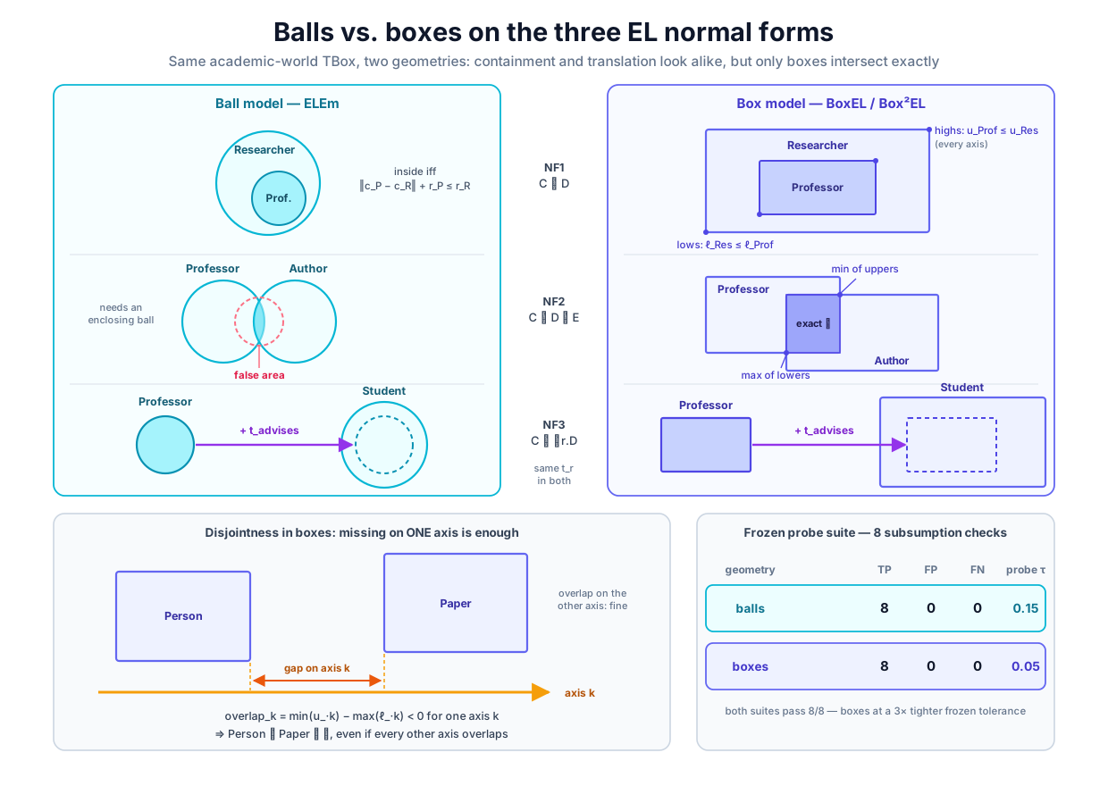The same three axiom shapes under both geometries: containment and translation look alike, but only the box column's intersection is the true region, and disjointness needs only one missed axis. Original diagram by the authors, created with AI assistance.

Training, and the committed head-to-head

Training is full-batch gradient descent, $\theta \leftarrow \theta - \eta\, \nabla_\theta L$ , on the three parameter blocks (centers, log-offsets, translations), from a seed-0 initialization, for 4000 epochs at learning rate $\eta = 0.05$ with a decay to $\eta/10$ after epoch 3800 so the final equilibrium settles to stable, quotable numbers (box_el.py lines 357–374). The committed trace shows the spring network relaxing (python3 box_el.py, section 3):

training — total squared-hinge loss and by axiom group (epoch 1 = untrained)
   epoch :      total |      NF1     NF2⊓     disj      NF3      NF4
       1 :   283.4835 | 121.3894   0.0000   0.0000  62.7180  99.3761
:    10.3909 |   6.2613   0.0000   0.0002   1.9388   2.1907
:     1.1293 |   0.3796   0.4096   0.0000   0.2306   0.1095
:     0.2988 |   0.1469   0.0257   0.0000   0.1068   0.0193
:     0.1465 |   0.0800   0.0174   0.0000   0.0488   0.0003
:     0.0943 |   0.0510   0.0149   0.0000   0.0284   0.0000
:     0.0804 |   0.0425   0.0150   0.0000   0.0228   0.0000
:     0.0678 |   0.0351   0.0150   0.0031   0.0146   0.0000

Read the columns, because they tell the chapter's story in miniature. The NF2 column starts at $0.0000$ not because conjunction is satisfied at initialization but because the randomly scattered boxes have an empty intersection, and an empty intersection satisfies its axiom vacuously; by epoch 50 the containment hinges have dragged boxes together, the intersection has become nonempty, and the NF2 loss briefly spikes to $0.4096$ before relaxing. And the total never reaches zero, for the same provable reason as last chapter: TenuredStudent must sit inside two boxes that the disjointness hinge holds apart, and a nonempty box cannot be empty, so its axioms keep a permanent violation, the geometric shadow of ⊥. That shadow explains why zero is unreachable, but it is not where most of the final $0.0678$ sits. As the committed trace itemizes it, the TenuredStudent cluster (its two containments, the TenuredStudentAdvisor existential, and the disjointness hinge they fight) is the provably unavoidable part of that residual, while the largest share sits on Researcher ⊑ Person against Person ⊓ _N1 ⊑ Researcher (_N1 is the fresh name normalization introduced for ∃authored.Paper), two jointly satisfiable axioms whose strict $\gamma$ margins pull the Researcher box in opposite directions: a spring compromise the equilibrium settles into, not a violation the logic forces, with the rest small spring compromise elsewhere. The disjointness column tells the same equilibrium story in miniature. It sits at zero through mid-training, then re-activates faintly at the end, because the trained boxes finish genuinely disjoint (the closure exhibit below prints a minimum overlap of $-0.0304$ ) but with less than the demanded $\gamma = 0.05$ of clearance, and $\lambda_\bot \max(0,\, -0.0304 + 0.05)^2 = 8 \cdot 0.0196^2 \approx 0.0031$ is exactly the table's final entry.

After training, the soundness probe accepts $A \sqsubseteq B$ exactly when the worst-axis protrusion of $A$ outside $B$ is within tolerance $\varepsilon$ (box_el.py lines 381–389):

def probe_gap(cen: np.ndarray, logoff: np.ndarray, a: str, b: str) -> float:
    """The worst-axis protrusion of box a outside box b:

        gap(A, B) = max_i max(l_B,i − l_A,i,  u_A,i − u_B,i).

    gap ≤ 0 means A is truly inside B; the probe accepts A ⊑ B iff gap ≤ ε."""

The probe scans the same 56 ordered pairs as the ball probe, with $\varepsilon = 0.05$ against the ball model's $\varepsilon = 0.15$ (el_embed.py line 55). The committed run prints the 8 gold subsumptions with their trained gaps, and then the centerpiece, the two-row confusion table (python3 box_el.py, sections 4–5):

4. soundness probe — accept A ⊑ B iff gap(A,B) = max_i max(l_B−l_A, u_A−u_B) ≤ ε = 0.05
   the 8 gold subsumptions, by their trained gaps:
     Dean       ⊑ Person      gap = -0.1048  ✓ contained
     Dean       ⊑ Professor   gap =  0.0199  ✓ contained
     Dean       ⊑ Researcher  gap = -0.0544  ✓ contained
     Professor  ⊑ Person      gap = -0.1000  ✓ contained
     Professor  ⊑ Researcher  gap = -0.0500  ✓ contained
     Researcher ⊑ Person      gap =  0.0000  ✓ contained
     Student    ⊑ Person      gap = -0.0500  ✓ contained
     Student    ⊑ Researcher  gap = -0.0500  ✓ contained
   scan of 8·7 = 56 ordered pairs: predicted 8, TP 8, FP 0, FN 0
   wrong pairs: none

5. balls vs boxes — the same 56-pair probe, same axioms, seed 0
   model            TP  FP  FN  precision  recall  probe slack
   balls (ELEm)      8   0   0     1.0000  1.0000  ε = 0.15
   boxes (BoxEL)     8   0   0     1.0000  1.0000  ε = 0.05

As a table, with the probe slack that each score was earned at:

model	TP	FP	FN	precision	recall	probe slack $\varepsilon$
balls (ELEm) [1]	8	0	0	1.0000	1.0000	0.15
boxes (BoxEL-style) [2]	8	0	0	1.0000	1.0000	0.05

The honest headline is a tie: on this 16-axiom TBox, both geometries recover the gold subsumptions perfectly. It would be easy, and wrong, to bury that. A 14-axiom ontology with 8 satisfiable named concepts simply does not have enough conjunction pressure to expose the ball model's approximation: of its two NF2 normal forms, one is the disjointness, leaving a single ordinary conjunction for the midpoint heuristic to satisfy, and one constraint in $\mathbb{R}^8$ leaves plenty of room to settle somewhere adequate. Three observations locate the real difference.

First, resist reading the probe-slack column as part of the score. Each suite's tolerance was set once and then frozen ( $\varepsilon = 0.15$ for balls, whose declaring comment says exactly that, el_embed.py lines 55–56; $\varepsilon = 0.05$ for boxes), so the column records a probe setting, not a measured need. The gold-gap list above shows why the distinction matters even inside a single row: six of the eight box gaps sit at or below $-0.0500$ , holding strictly with the full training margin $\gamma$ of room, yet Dean ⊑ Professor protrudes by $0.0199$ and passes only because the slack is there to spend. The two tolerances say which ruler each model was measured with, not which one needed help.

Second, the advantage is structural, visible in the losses rather than the scores: the box NF2 loss trains the exact intersection against $C$ , while the ball NF2 loss trains a proxy. The failure mode of the proxy is not randomness but systematic false area, and it compounds with the number and depth of conjunctions.

Third, that compounding is exactly what the published record shows at scale. On the standard ontology benchmarks (GALEN, the Gene Ontology, and Anatomy), where thousands of NF2 axioms exercise the intersection, the box-based models report gains over the ball baseline on most benchmark and metric combinations: BoxEL over ELEm [2], and Box²EL ahead of the whole baseline set, the ELEm ball model, BoxEL, and ELBE included, on the bulk of the reported settings [4]. ELBE makes the same intersectional-closure argument, but reports its own gains not on these three ontologies: it is evaluated on a synthetic conjunction task and protein-interaction prediction, where its largest jump lands squarely on the conjunction metric [3]. The toy tie and the published gap are the same phenomenon read at two scales: faithfulness to ⊓ is a geometry property before it is a training property, and it starts costing accuracy exactly when the ontology exercises it.

The closure exhibit: a trained intersection, corner by corner

The confusion table compares verdicts. The closure exhibit compares objects. After training, the run takes the Professor and Researcher boxes and computes their intersection by the corner arithmetic, then prints all four corner vectors (python3 box_el.py, section 6):

6. closure — Professor ⊓ Researcher by corner arithmetic IS a box
   axis              1       2       3       4       5       6       7       8
   inter lo     -0.643   0.151  -0.151  -0.317  -0.222  -0.125   0.154   0.360
   inter hi     -0.205   0.429   0.312   0.179   0.253   0.314   0.627   0.810
   Prof  lo     -0.643   0.151  -0.151  -0.317  -0.222  -0.125   0.154   0.360
   Prof  hi     -0.205   0.429   0.312   0.179   0.253   0.314   0.627   0.810
   the model learned Professor ⊑ Researcher, so the intersection ≈ the Professor box
   (Professor ⊓ Researcher ≡ Professor) — whereas two balls intersect in a lens that
   is NOT a ball: boxes_vs_balls.py measures 60.56% false-positive area for the best
   enclosing ball, and here the corner arithmetic is exact with zero false area

   Professor/Student disjointness, exactly: min per-axis overlap = -0.0304 < 0

Read the numbers down each column: the intersection's corners coincide with Professor's on every axis, to the printed precision. That is the logic showing through the geometry. Volume 2's reasoner derived Professor ⊑ Researcher, the training realized it as containment, and containment makes the intersection identity $X \cap Y = X$ (for $X \subseteq Y$ ) hold in coordinates: on every axis, Professor's lower corner is the larger lower and its upper corner the smaller upper, so the max/min arithmetic returns Professor's own corners. The printed region is a genuine, queryable concept, $\mathrm{box}(\text{Professor} \sqcap \text{Researcher})$ , with zero false area, where the ball model's best effort on the same conjunction carried 60.56% provably false area. And the last line closes the disjointness ledger: the trained Professor and Student boxes have a minimum per-axis overlap of $-0.0304$ , a strict miss on at least one axis, so the ⊑ ⊥ axiom holds exactly in the trained geometry, not merely up to tolerance. The module's competency asserts pin all of this on every run: 15 trained axioms plus 1 skipped chain, 8 of 8 gold recovered, recall at least the balls' recall, negative minimum overlap, and a nonempty intersection box (box_el.py lines 441–453).

Box²EL: bumps, role boxes, and the many-to-many fix

One weakness survives everything above, and the previous chapter already met it: a role is a single translation vector. Every axiom that routes through advises must reuse the same $t_{\text{advises}}$ , so if Dean ⊑ ∃advises.Professor and Professor ⊑ ∃advises.Student both hold, one arrow must carry the Dean box into the Professor box and the Professor box into the Student box, and the spring compromise between those demands is where residual NF3 loss lives. This is the ontology-level twin of TransE's one-to-many collapse from Translational Models, and Box²EL is the published fix [4]. It changes the role vocabulary twice. First, every concept $A$ carries, besides its box, a bump vector $b_A \in \mathbb{R}^d$ , and the existential $A \sqsubseteq \exists r.B$ is scored with the filler's bump added to the source: the same role lands differently for different fillers, because the translation the source box undergoes is shifted by $b_B$ . A single role can then relate many concept pairs without forcing all of them onto one shared offset. Second, the role $r$ itself becomes a pair of role boxes (a head box and a tail box) rather than a point translation, so membership in the domain and range of $r$ is region containment like everything else, and the model can express that a role's sources and targets each occupy a region of space with volume, not a direction. On the toy TBox none of this is needed, which is why the companion keeps the translation-only core (its docstring says so, box_el.py lines 13–15); at GALEN, Gene Ontology, and Anatomy scale, the WWW '24 evaluation reports that these two changes improve subsumption prediction over BoxEL, ELBE, and the ball baseline on the bulk of the benchmark suite [4]. The pattern to carry forward: each geometric enrichment (ball → box → box with bumps) buys back a piece of the logic that the previous geometry silently approximated.

The unsolved part

The probe this chapter and the last one share has a quiet blind spot, and naming it honestly reframes what "faithful" must mean. The probe tests subsumptions between named concepts: 56 ordered pairs of atomic names, judged against the reasoner. Recall on that set is necessary for faithfulness, but it is not sufficient, because EL++ does not only entail statements about names. It entails statements about concepts composed of constructors: does the trained geometry get $A \sqcap B \sqsubseteq C$ right for pairs the TBox never mentioned together? Does $\exists r.(A \sqcap B)$ land where the logic says it must? A perfect score on atomic pairs is compatible with systematic error on composed ones, and the very closure property this chapter celebrated is what makes the question sharp: because $\mathrm{box}(A) \cap \mathrm{box}(B)$ is a box, the geometry assigns a definite region to every conjunction, including the untrained ones, and each of those regions is a checkable claim. Balls could not even be interrogated this way; boxes can, so they inherit the obligation. What is needed is a model whose construction guarantees, not merely encourages, that the region assigned to a complex concept is computed from its parts in a way that preserves entailment across the full EL++ constructor set: closure not as an exhibit at the end of training but as an invariant of the representation. That is an open design problem in general, and the subject of the next chapter in particular.

Why it matters

For the neuro-symbolic program, this chapter upgrades a slogan into a measurement protocol. "Embeddings should respect the ontology" is vague; "train the exact intersection box against its superconcept, then score the trained geometry against the reasoner's classification, row for row against a controlled baseline" is an experiment, and the committed run is its instance. Two lessons transfer forward. First, choose the geometry to match the algebra of the logic: the reason NF2 became exact was not a better optimizer or a bigger model but a representation closed under the operation the axiom talks about; the same principle will pick the geometry for query conjunction in complex query answering and for the differentiable operators of Volume 4. Second, faithfulness has a budget you can locate: the residual loss itemizes axiom by axiom into a provably unavoidable part (the geometric shadow of the unsatisfiable TenuredStudent) and a $\gamma$ -margin spring compromise between jointly satisfiable axioms, so the error is not merely small, it is attributable, and each part can be traced to its cause. When Volume 4 attaches losses like these to neural predictors, so that a perception model is penalized for violating a TBox, the quality of that supervision is precisely the quality measured here: a loss that speaks the logic's own language transmits the logic; a loss that approximates it transmits the approximation.

Key terms

Axis-aligned box — a product of $d$ intervals $[c_i - o_i,\, c_i + o_i]$ , parameterized by a center $c$ and positive half-widths $o = e^{w}$ ; the concept shape of BoxEL-style models.
Lower / upper corner — the vectors $l = c - o$ and $u = c + o$ ; all containment, intersection, and disjointness conditions in this chapter are inequalities on corners.
Inclusion violation (per-corner hinge) — the loss $\sum_i \max(0, l_{B,i} - l_{A,i} + \gamma)^2 + \sum_i \max(0, u_{A,i} - u_{B,i} + \gamma)^2$ , zero exactly when $\mathrm{box}(A)$ sits inside $\mathrm{box}(B)$ with margin $\gamma$ on every side.
Squared hinge — squaring each violation makes the gradient proportional to the violation, so opposing constraints relax like springs instead of stalling in the constant-magnitude, per-coordinate cancellations the L1 hinge permits.
Intersectional closure — the property that the intersection of two boxes is a box, with corners $l_I = \max(l_A, l_B)$ , $u_I = \min(u_A, u_B)$ ; it lets NF2 train the exact object the axiom mentions [3].
Vacuous satisfaction — the convention that an NF2 axiom whose intersection box is empty ( $l_{I,i} \gt u_{I,i}$ on some axis) contributes zero loss and zero gradient, because $\varnothing \subseteq C$ is logically true.
Overlap / missed axis — the per-axis quantity $\mathrm{ov}_i = \min(u_{A,i}, u_{B,i}) - \max(l_{A,i}, l_{B,i})$ ; boxes are disjoint exactly when $\mathrm{ov}_i \lt 0$ for some $i$ , so disjointness training hinges only the smallest overlap.
Probe gap — $\mathrm{gap}(A,B) = \max_i \max(l_{B,i} - l_{A,i},\, u_{A,i} - u_{B,i})$ , the worst-axis protrusion of $A$ outside $B$ ; the probe accepts $A \sqsubseteq B$ iff the gap is at most $\varepsilon$ .
Bump vector (Box²EL) — a per-concept vector added to the source of an existential so the same role can land differently for different fillers, the ontology-level fix for one-translation-per-role [4].
Role box (Box²EL) — a head/tail pair of boxes representing a role's sources and targets as regions rather than a single point translation [4].

Where this leads

The unsolved part named the gap: recall on atomic subsumptions is necessary, not sufficient, and the constructor set is where faithfulness is really decided. The next chapter, TransBox and mOWL, takes both halves of that sentence seriously. TransBox is a construction aimed at closure under the full EL++ concept grammar, so that complex concepts get regions by construction rather than by luck; and mOWL is the tooling that turns the experiments this Part has been hand-building (load an ontology, normalize it, train a geometric model, evaluate against a reasoner) into a standard, reproducible workflow at the scale of SNOMED CT and the Gene Ontology. The question travels intact: not "can the geometry memorize the TBox?" but "does the geometry compute the logic?"

Companion code: examples/neural/box_el.py trains the box model on the same 15 normal-form axioms as examples/neural/el_embed.py (both import Volume 2's examples/symbolic/el_completion.py for normalization and the gold classification), runs the 56-pair soundness probe for both geometries in one process, and prints the head-to-head table, the closure exhibit, and the disjointness check quoted above. Run python3 box_el.py from examples/neural/ to reproduce every number in this chapter; seed 0 makes the output byte-identical across runs, and the competency asserts in run() fail the process if any quoted claim stops holding.

What this chapter covers​

Same experiment, one changed variable​

The model: a concept is a box, a role is a translation​

Box inclusion, derived corner by corner​

NF2 finally exact: the intersection is a box​

Existentials as translation, disjointness as a missed axis​

Training, and the committed head-to-head​

The closure exhibit: a trained intersection, corner by corner​

Box²EL: bumps, role boxes, and the many-to-many fix​

The unsolved part​

Why it matters​

Key terms​

Where this leads​