Bilinear Models: DistMult and ComplEx

📍 Where we are: Part I · Knowledge Graph Embeddings — Chapter 3. Translational Models bet that a relation is a displacement and paid for it with the 1-to-many collapse; this chapter changes the verb from add to multiply and meets a different, sharper failure.

The last chapter ended with a model that walks: a triple is plausible when the head's point, pushed along the relation's arrow, lands near the tail's point. This chapter replaces walking with a fundamentally different geometric verb. A bilinear model scores a triple by multiplying coordinates together and adding up the products, so that a fact is plausible when head, relation, and tail agree, dimension by dimension, rather than when two points sit close together. Multiplication buys real things that translation cannot deliver, including the ability to represent a symmetric relation without collapsing its endpoints. But the simplest multiplicative model, DistMult, buys them at a price we can state as a theorem and prove in two lines: its score cannot distinguish a triple from its reversal, ever, for any setting of the parameters. Our graph contains a relation for which that is fatal. The fact (p2, cites, p1) is true and its reverse is false, and the committed run will show DistMult assigning both directions the bitwise identical score. The repair, ComplEx, keeps the multiplicative form and changes exactly one thing: the vectors become complex-valued and the tail is conjugated. That conjugation flips one sign in the expanded score, the flipped sign makes the score direction-aware, and the same run shows the two citation directions coming apart by more than eleven points. Every loss and every gradient in between is derived by hand and checked against the committed code, and every number is quoted from a real run.

The simple version

Imagine a matchmaking service that scores a proposed pairing with a questionnaire. Every entity has filled in sixteen sliders, and every relation is a rubric that says how much each question matters. To score "does p2 cite p1," you take question 1, multiply p2's answer times the rubric's weight times p1's answer, do the same for all sixteen questions, and add everything up. Big positive products mean the three agree; the sum is the score. Now notice the flaw: the rubric has no idea which questionnaire came from the head and which from the tail. Multiplication does not care about order, so "p2 cites p1" and "p1 cites p2" produce exactly the same sixteen products and exactly the same sum. For a two-way relation like "collaborates" that is fine, even ideal. For a one-way relation like "cites" it is hopeless. ComplEx's fix is to give every question two channels, and to read the tail's second channel through a sign flip, like grading the tail against a mirrored answer key. Head and tail are now processed differently, so swapping them changes the score, and direction becomes something the model can learn.

What this chapter covers

• The general bilinear score: RESCAL's $\mathbf{e}_h^\top W_r \mathbf{e}_t$ with a full $d \times d$ matrix per relation, expanded into its double sum, and the parameter bill that motivates cutting it down.
• The diagonal restriction: DistMult keeps only the matrix diagonal, collapsing the double sum to $\sum_i e_h[i]\, w_r[i]\, e_t[i]$, with a parameter-count table across TransE, RESCAL, DistMult, and ComplEx.
• The symmetry theorem, proved: commutativity of real multiplication makes the diagonal score invariant under swapping head and tail, for every relation and every parameter setting; the committed run shows the tie on cites to the last bit.
• Complex vectors, gently: $\mathbb{C}^d$ as a pair of real vectors, the conjugate, and ComplEx's score $\mathrm{Re}\langle \mathbf{e}_h, \mathbf{w}_r, \overline{\mathbf{e}_t} \rangle$ expanded step by step into four real terms, where the one minus sign that restores direction is visible.
• The logistic loss and every gradient: $L = \mathrm{softplus}(-y\,s)$, the derivative $\partial L/\partial s = -y\,\sigma(-y\,s)$ built link by link through the chain rule, the three DistMult partials and the six ComplEx partials, the L2 weight-decay update, and a central-difference check that confirms every formula to within $2 \times 10^{-10}$.
• The committed head-to-head: both training-loss curves, the symmetry table (DistMult 4.8879 versus 4.8879; ComplEx 6.6413 versus −4.5805), and the filtered ranking results, all real numbers from the deterministic run.
• What multiplication buys: symmetric relations without collapse, a per-relation dial between symmetry and antisymmetry, and the full-expressiveness guarantee for ComplEx.
• The unsolved part: a score over point embeddings ranks single edges, but concepts and query answers are sets, and points have no geometry of containment; Part II gives sets their own shapes.

From walking to multiplying: the general bilinear score

Recall the shape of the problem. Each of the 13 entities of the academic graph gets an entity embedding, a vector of $d$ real numbers (the embedding dimension; the companion code again uses $d = 16$). What changes is what a relation gets. TransE gave it a vector to add. The bilinear family gives it a table of interaction weights: a full $d \times d$ relation matrix $W_r$, one row and one column per embedding dimension, whose entry $W_r[i,j]$ says how much the head's coordinate $i$ interacting with the tail's coordinate $j$ counts as evidence for relation $r$. The score is the bilinear form

$$s(h, r, t) \;=\; \mathbf{e}_h^\top W_r\, \mathbf{e}_t \;=\; \sum_{i=1}^{d} \sum_{j=1}^{d} e_h[i]\; W_r[i,j]\; e_t[j],$$

where the superscript $\top$ is the transpose, which turns the column vector $\mathbf{e}_h$ into a row so the matrix product is defined, and the indices $i$ and $j$ each run over the $d$ coordinates. Read the double sum from the inside out: form every one of the $d^2$ pairwise products of a head coordinate with a tail coordinate, weight each pair by the matrix entry that governs it, and add everything up. "Bilinear" is the precise name for this shape: freeze $\mathbf{e}_t$ and the score is a linear function of $\mathbf{e}_h$; freeze $\mathbf{e}_h$ and it is linear in $\mathbf{e}_t$; linear in each argument separately, hence bi-linear.

This is the model called RESCAL, and it comes with a useful second reading [1]. Stack the whole graph into a three-way array (a tensor) $X$ with one 0/1 entry per possible triple, so $X[h, r, t] = 1$ exactly when the fact holds. Then asking the embeddings to make $s(h,r,t)$ large for true triples and small for false ones is asking for a tensor factorization: an approximation $X[h,r,t] \approx \mathbf{e}_h^\top W_r \mathbf{e}_t$ that rebuilds the incidence tensor from a small set of shared factors. Link prediction becomes the factorization's generalization: entries of $X$ we never observed are predicted by the same low-dimensional factors that reconstruct the entries we did.

The trouble is the bill. Every relation carries its own $d \times d$ matrix, and matrices are quadratically expensive. On our tiny graph at $d = 16$, each relation costs $16^2 = 256$ numbers and the 5 relation matrices already cost $5 \times 256 = 1280$, dwarfing the $13 \times 16 = 208$ the entities cost; on a real graph with thousands of relations and $d$ in the hundreds, the relation matrices dominate everything and overfit long before they converge. The natural response is to constrain $W_r$, and the simplest constraint that keeps the multiplicative character is the subject of the next section.

The diagonal restriction: DistMult

DistMult keeps only the diagonal of the relation matrix [2]. Formally, require $W_r = \mathrm{diag}(\mathbf{w}_r)$: a matrix that is zero everywhere except the entries $W_r[i,i] = w_r[i]$ running down its main diagonal, so each relation is once again described by just $d$ numbers. Substituting into the double sum, every term with $i \neq j$ has $W_r[i,j] = 0$ and vanishes, and only the $d$ matched-index terms survive:

$$s(h, r, t) \;=\; \sum_{i=1}^{d} \sum_{j=1}^{d} e_h[i]\; W_r[i,j]\; e_t[j] \;=\; \sum_{i=1}^{d} e_h[i]\; w_r[i]\; e_t[i].$$

The score is a three-way inner product: coordinate by coordinate, multiply the head's value, the relation's weight, and the tail's value, then sum. Each dimension is a latent feature; a triple scores high when there are dimensions where all three light up together, positive-times-positive-times-positive (or with an even number of negatives), and the relation vector $\mathbf{w}_r$ says which dimensions the relation cares about and with what sign. The committed implementation is a single return line, and its docstring announces the trouble the next section proves (bilinear.py lines 57–65):

def distmult_score(ent: np.ndarray, rel: np.ndarray,
                   hi: int, ri: int, ti: int) -> float:
    """DistMult's score  s(h, r, t) = Σ_i e_h[i] · w_r[i] · e_t[i].

    Because elementwise multiplication commutes, s(h, r, t) = s(t, r, h) for
    every choice of parameters — the symmetry defect demonstrated below.  The
    grouping w_r ⊙ (e_h ⊙ e_t) makes that equality exact even in floating
    point: swapping h and t produces the bitwise-identical product array."""
    return float(np.sum(rel[ri] * (ent[hi] * ent[ti])))

The parameter arithmetic now favors DistMult decisively. Here is the full bill for our graph, 13 entities and 5 relations at 16 real dimensions per row, with each model's relation representation made explicit. In the table, the symbol $\in$ reads "is an element of," $\mathbb{R}^{16}$ is the set of vectors of 16 real numbers, $\mathbb{R}^{16 \times 16}$ the set of 16-by-16 real matrices, and $\mathbb{C}^{8}$ the set of vectors of 8 complex numbers (a notion unpacked two sections below):

model	relation representation	params per relation	total on our graph	handles symmetric $r$	handles antisymmetric $r$
TransE	translation vector $\mathbf{w}_r \in \mathbb{R}^{16}$	16	$208 + 80 = 288$	only by collapse	yes
RESCAL	full matrix $W_r \in \mathbb{R}^{16 \times 16}$	256	$208 + 1280 = 1488$	yes	yes
DistMult	diagonal $\mathbf{w}_r \in \mathbb{R}^{16}$	16	$208 + 80 = 288$	always (forced)	never
ComplEx	complex vector $\mathbf{w}_r \in \mathbb{C}^{8}$	16 real	$208 + 80 = 288$	yes ($\mathbf{w}_{\mathrm{im}} = 0$)	yes ($\mathbf{w}_{\mathrm{re}} = 0$)

DistMult matches TransE's 288 parameters exactly while keeping RESCAL's multiplicative interactions, and on the standard benchmarks of its era it was surprisingly strong [2]. But look again at the last two columns of the table. The word "forced" in DistMult's row and the word "never" beside it are the two ends of one theorem, and it is short enough to prove right now.

The symmetry theorem

Theorem. For every choice of entities $h$ and $t$, every relation $r$, and every possible value of the embedding parameters, DistMult's score satisfies $s(h, r, t) = s(t, r, h)$.

Proof. Fix any dimension $i$. The $i$-th summand of $s(h,r,t)$ is the product of three real numbers, $e_h[i] \cdot w_r[i] \cdot e_t[i]$. Multiplication of real numbers is commutative, meaning $ab = ba$ for all reals $a$ and $b$, so the three factors can be reordered freely: $e_h[i]\, w_r[i]\, e_t[i] = e_t[i]\, w_r[i]\, e_h[i]$. This holds for each $i$ separately, and summing equal terms gives equal sums:

$$s(h, r, t) \;=\; \sum_{i=1}^{d} e_h[i]\, w_r[i]\, e_t[i] \;=\; \sum_{i=1}^{d} e_t[i]\, w_r[i]\, e_h[i] \;=\; s(t, r, h). \qquad \blacksquare$$

Notice what the theorem does not say. It does not say DistMult tends to confuse directions, or struggles with them, or needs more data to learn them. It says the two scores are the same function of the parameters. There is no gradient step, no dataset, no training schedule, no dimension count under which they differ, because they are equal as algebraic expressions before any number is filled in. The identity even survives floating-point arithmetic in the committed code: the grouping rel[ri] * (ent[hi] * ent[ti]) computes $\mathbf{w}_r \odot (\mathbf{e}_h \odot \mathbf{e}_t)$, where $\odot$ is the Hadamard product, elementwise multiplication of vectors, so $(\mathbf{a} \odot \mathbf{b})[j] = a[j]\,b[j]$. Swapping $h$ and $t$ swaps the two factors of the inner Hadamard product, which NumPy multiplies commutatively, so the product array is bitwise identical and the two scores agree to the last bit (bilinear.py lines 61–65).

The consequence, on our own graph

Our graph has exactly the relation this theorem punishes. The cites relation holds from a citing paper to a cited one: the training set contains (p2, cites, p1) and (p3, cites, p2), and citation is antisymmetric, since a paper published later cites an earlier one and never the converse. A model doing its job should score (p2, cites, p1) high and (p1, cites, p2) low. The theorem says DistMult cannot, even in principle: whatever score training earns for the true direction is inherited, identically, by the false one. Here is the committed demonstration, printed after both models train for 1000 epochs (the second column belongs to ComplEx, which we build next; hold it for a page):

the symmetry problem: `cites` is antisymmetric, and only the
forward direction (p2, cites, p1) was ever trained as true
  score                        DistMult    ComplEx
  s(p2, cites, p1)   true       4.8879     6.6413
  s(p1, cites, p2)   false      4.8879    -4.5805
  |forward - reverse|          0.0000     11.2217

The DistMult column is the theorem made empirical: forward and reverse are 4.8879 and 4.8879, and the harness does not merely print the tie, it asserts it, requiring the absolute difference to be below $10^{-9}$ (bilinear.py line 332); the run's summary line reports the measured difference as 0.0e+00, exact to the bit for the reason just given. Training raised both directions together, like two ends of one plank. And the failure is self-reinforcing: every gradient that pushes the true fact's score up pushes the false reverse up by exactly the same amount, because equal functions have equal gradients.

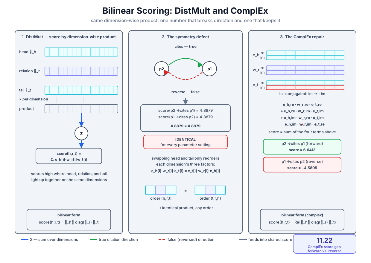Bilinear scoring in one picture: DistMult multiplies head, relation, and tail dimension by dimension and sums (left), which makes the score provably blind to direction (middle); ComplEx splits each dimension into real and imaginary channels and conjugates the tail, and the one flipped sign separates the two citation directions by 11.22 (right). Original diagram by the authors, created with AI assistance.

Complex vectors, gently

The repair needs one piece of freshman algebra back on the table. A complex number is a pair of real numbers written $z = a + b\,\mathrm{i}$, where $\mathrm{i}$ is a formal symbol obeying the single rule $\mathrm{i}^2 = -1$; the number $a$ is the real part and $b$ the imaginary part. Two complex numbers multiply by ordinary distribution plus that one rule, and it is worth doing once in full because the expansion of ComplEx's score is this computation three factors deep:

$$(a + b\,\mathrm{i})(c + d\,\mathrm{i}) \;=\; ac + ad\,\mathrm{i} + bc\,\mathrm{i} + bd\,\mathrm{i}^2 \;=\; (ac - bd) + (ad + bc)\,\mathrm{i},$$

where the last step used $\mathrm{i}^2 = -1$ to fold the $bd$ term into the real part with a minus sign. The conjugate of $z$, written $\overline{z}$, flips the sign of the imaginary part: $\overline{a + b\,\mathrm{i}} = a - b\,\mathrm{i}$. Conjugation is the only operation in this chapter that treats the two channels of a complex number asymmetrically, and that asymmetry is the entire trick.

A complex vector $\mathbf{u} \in \mathbb{C}^k$ (the set of lists of $k$ complex numbers) is nothing exotic in code: it is stored as two real vectors of length $k$, one holding the real parts and one the imaginary parts. The committed implementation does exactly this, keeping arrays e_re, e_im, w_re, w_im, and it splits the same budget as DistMult: $d = 16$ real dimensions read as $k = d/2 = 8$ complex ones (bilinear.py lines 37 and 261–265), so the parameter totals in the table above match at 288.

ComplEx: conjugate the tail

ComplEx keeps DistMult's three-way product and changes one factor [3]. Define the trilinear product of three complex vectors as the sum of their elementwise products, $\langle \mathbf{u}, \mathbf{v}, \mathbf{w} \rangle = \sum_i u_i\, v_i\, w_i$, a complex number. ComplEx scores a triple by conjugating the tail and keeping the real part (written $\mathrm{Re}(\cdot)$, the function that extracts a complex number's real component):

$$s(h, r, t) \;=\; \mathrm{Re}\,\big\langle \mathbf{e}_h,\; \mathbf{w}_r,\; \overline{\mathbf{e}_t} \big\rangle \;=\; \mathrm{Re} \sum_{i=1}^{k} e_h[i]\; w_r[i]\; \overline{e_t[i]}.$$

To see what this actually computes, expand one summand into real and imaginary parts, writing $h_{\mathrm{re}}, h_{\mathrm{im}}$ for the two channels of $e_h[i]$ and likewise for the relation and tail (all six symbols are real numbers; the dimension index is suppressed). The factor being multiplied is $(h_{\mathrm{re}} + h_{\mathrm{im}}\mathrm{i})(w_{\mathrm{re}} + w_{\mathrm{im}}\mathrm{i})(t_{\mathrm{re}} - t_{\mathrm{im}}\mathrm{i})$, the minus sign in the last factor being the conjugation. Multiply the first two factors using the product rule derived above:

$$(h_{\mathrm{re}} + h_{\mathrm{im}}\mathrm{i})(w_{\mathrm{re}} + w_{\mathrm{im}}\mathrm{i}) \;=\; (h_{\mathrm{re}} w_{\mathrm{re}} - h_{\mathrm{im}} w_{\mathrm{im}}) \;+\; (h_{\mathrm{re}} w_{\mathrm{im}} + h_{\mathrm{im}} w_{\mathrm{re}})\,\mathrm{i}.$$

Now multiply this by $(t_{\mathrm{re}} - t_{\mathrm{im}}\mathrm{i})$ and keep only the real part. A real part arises two ways: real-times-real, and imaginary-times-imaginary through $\mathrm{i} \cdot (-\mathrm{i}) = +1$:

$$\mathrm{Re}(\cdots) \;=\; (h_{\mathrm{re}} w_{\mathrm{re}} - h_{\mathrm{im}} w_{\mathrm{im}})\, t_{\mathrm{re}} \;+\; (h_{\mathrm{re}} w_{\mathrm{im}} + h_{\mathrm{im}} w_{\mathrm{re}})\, t_{\mathrm{im}}.$$

Distribute the two products and the score's per-dimension contribution lands in exactly four real terms:

$$w_{\mathrm{re}} h_{\mathrm{re}} t_{\mathrm{re}} \;+\; w_{\mathrm{re}} h_{\mathrm{im}} t_{\mathrm{im}} \;+\; w_{\mathrm{im}} h_{\mathrm{re}} t_{\mathrm{im}} \;-\; w_{\mathrm{im}} h_{\mathrm{im}} t_{\mathrm{re}}.$$

This is precisely what the committed code computes, and its docstring says where the crucial sign comes from (bilinear.py lines 99–115):

def complex_score(ent_re: np.ndarray, ent_im: np.ndarray,
                  rel_re: np.ndarray, rel_im: np.ndarray,
                  hi: int, ri: int, ti: int) -> float:
    """ComplEx's score  s = Re(⟨e_h, w_r, conj(e_t)⟩), expanded over the real
    (``_re``) and imaginary (``_im``) parts into its four real terms:

        s = Σ_i [  w_re·h_re·t_re  +  w_re·h_im·t_im
                 + w_im·h_re·t_im  −  w_im·h_im·t_re ]

    The last term's minus sign comes from conj(e_t) = t_re − i·t_im; it is the
    only asymmetry in the formula, and it is what lets ComplEx score
    (p2, cites, p1) and (p1, cites, p2) differently."""
    h_re, h_im = ent_re[hi], ent_im[hi]
    w_re, w_im = rel_re[ri], rel_im[ri]
    t_re, t_im = ent_re[ti], ent_im[ti]
    return float(np.sum(w_re * h_re * t_re + w_re * h_im * t_im
                        + w_im * h_re * t_im - w_im * h_im * t_re))

Now regroup the four terms by which relation channel they use, because the grouping exposes the model's structure. The two $w_{\mathrm{re}}$ terms and the two $w_{\mathrm{im}}$ terms collect into

$$s(h,r,t) \;=\; \sum_{i=1}^{k} w_{\mathrm{re}}[i]\,\big(h_{\mathrm{re}}[i]\, t_{\mathrm{re}}[i] + h_{\mathrm{im}}[i]\, t_{\mathrm{im}}[i]\big) \;+\; \sum_{i=1}^{k} w_{\mathrm{im}}[i]\,\big(h_{\mathrm{re}}[i]\, t_{\mathrm{im}}[i] - h_{\mathrm{im}}[i]\, t_{\mathrm{re}}[i]\big).$$

Swap $h$ and $t$ and watch each bracket. The first bracket, $h_{\mathrm{re}} t_{\mathrm{re}} + h_{\mathrm{im}} t_{\mathrm{im}}$, maps to $t_{\mathrm{re}} h_{\mathrm{re}} + t_{\mathrm{im}} h_{\mathrm{im}}$, the same expression: it is symmetric under the swap. The second bracket, $h_{\mathrm{re}} t_{\mathrm{im}} - h_{\mathrm{im}} t_{\mathrm{re}}$, maps to $t_{\mathrm{re}} h_{\mathrm{im}} - t_{\mathrm{im}} h_{\mathrm{re}}$, which is its exact negation: it is antisymmetric. Subtracting the swapped score from the original, the symmetric parts cancel and the antisymmetric parts double:

$$s(h, r, t) - s(t, r, h) \;=\; 2 \sum_{i=1}^{k} w_{\mathrm{im}}[i]\,\big(h_{\mathrm{re}}[i]\, t_{\mathrm{im}}[i] - h_{\mathrm{im}}[i]\, t_{\mathrm{re}}[i]\big).$$

Every relation therefore owns a dial. Set $\mathbf{w}_{\mathrm{im}} = \mathbf{0}$ and the difference vanishes for all entity pairs: the relation is perfectly symmetric, and the score reduces to a DistMult-style sum over the doubled channels, with the relation weight $w_{\mathrm{re}}[i]$ shared by each dimension's two channels; zero the entity imaginary parts as well and what remains is exactly a $k$-dimensional DistMult, so ComplEx contains DistMult as the special case of purely real embeddings. Set $\mathbf{w}_{\mathrm{re}} = \mathbf{0}$ and only the antisymmetric part survives, giving $s(h,r,t) = -s(t,r,h)$: a perfectly antisymmetric relation. Training tunes each relation's two channels independently, so collaborates-style relations and cites-style relations can coexist in one model, each landing where the data pushes it on the symmetry spectrum. One conjugation bought the whole dial.

The loss and every gradient, by hand

Both models train identically, so the derivation pays for itself twice. Each of the 15 training triples is a positive with label $y = +1$; each is paired, per epoch, with one uniformly sampled corruption carrying $y = -1$, resampled whenever the corruption is itself a known-true triple, the same trap and the same fix as the last chapter (bilinear.py lines 215–227). The per-example objective is the logistic loss:

$$L \;=\; \mathrm{softplus}(-y\,s) \;=\; \ln\!\big(1 + e^{-y\,s}\big),$$

where $\ln$ is the natural logarithm (the inverse of the exponential, so $\ln e^x = x$) and $\mathrm{softplus}(x) = \ln(1 + e^x)$ is the smooth ramp: near zero for large negative $x$, close to $x$ itself for large positive $x$. To read the loss, recall from Volume 1 that $\sigma(x) = 1/(1 + e^{-x})$ is the sigmoid, and note the identity $-\ln \sigma(x) = -\ln\frac{1}{1+e^{-x}} = \ln(1 + e^{-x}) = \mathrm{softplus}(-x)$. So $L = -\ln \sigma(y\,s)$: if we read $\sigma(s)$ as the model's probability that the triple is true, then $\sigma(y\,s)$ is the probability it assigns to the correct label, and the loss is the negative log-likelihood of being right. A positive scored high, or a negative scored low, makes $y\,s$ large and the loss nearly zero; a confident mistake makes $y\,s$ very negative and the loss grows linearly, like the un-clamped side of a hinge. The code computes it stably as np.logaddexp(0.0, -y * s), which is $\ln(e^0 + e^{-ys})$ evaluated without overflow (bilinear.py line 85).

The chain through the score. The gradient of $L$ with respect to any parameter factors through $s$, so first differentiate the softplus. One calculus fact does the work: the natural logarithm differentiates as $\frac{d}{dv}\ln v = \frac{1}{v}$, so the chain rule gives $\frac{d}{du}\ln v(u) = \frac{v'(u)}{v(u)}$ for any inner function $v$; here the inner function is $v(u) = 1 + e^u$, whose derivative is $e^u$. With $u = -y\,s$,

$$\frac{d}{du}\,\mathrm{softplus}(u) \;=\; \frac{d}{du} \ln(1 + e^u) \;=\; \frac{e^u}{1 + e^u} \;=\; \frac{1}{e^{-u} + 1} \;=\; \sigma(u),$$

where the second step applied $\frac{d}{du}\ln v = \frac{v'}{v}$ and the third step multiplied numerator and denominator by $e^{-u}$. The softplus's derivative is the sigmoid. Now the chain rule through $u = -y\,s$, whose derivative in $s$ is the constant $-y$; the symbol $\partial$ marks a partial derivative, the rate of change with respect to the named variable while every other argument is held fixed:

$$\frac{\partial L}{\partial s} \;=\; \sigma(-y\,s) \cdot \frac{\partial(-y\,s)}{\partial s} \;=\; -\,y\,\sigma(-y\,s).$$

This is dl_ds = -y * _sigmoid(-y * s) verbatim (bilinear.py lines 86–87). It is the same clean error signal that the sigmoid and cross-entropy produced together in Volume 1. Seeing that takes one reflection identity for the sigmoid:

$$\sigma(-s) \;=\; \frac{1}{1 + e^{s}} \;=\; \frac{e^{-s}}{e^{-s} + 1} \;=\; \frac{(e^{-s} + 1) - 1}{e^{-s} + 1} \;=\; 1 - \frac{1}{1 + e^{-s}} \;=\; 1 - \sigma(s),$$

where the second step multiplied numerator and denominator by $e^{-s}$, the third step rewrote the numerator as the denominator minus one, and splitting that fraction leaves one minus the sigmoid's defining expression. So for $y = +1$ the gradient $-\sigma(-s)$ equals $\sigma(s) - 1$, and for $y = -1$ it is $\sigma(s)$ directly, that is $\sigma(s) - 0$; writing $p = \sigma(s)$ and recoding the label into $\tilde{y} \in \{0, 1\}$ gives $\partial L / \partial s = p - \tilde{y}$, prediction minus target.

DistMult's three partials. The score $s = \sum_i e_h[i]\, w_r[i]\, e_t[i]$ is a sum in which each coordinate $e_h[j]$ of the head appears in exactly one term, the $j$-th, and appears there linearly with coefficient $w_r[j]\, e_t[j]$. Differentiating a linear function reads off its coefficient:

$$\frac{\partial s}{\partial e_h[j]} = w_r[j]\, e_t[j], \qquad \frac{\partial s}{\partial w_r[j]} = e_h[j]\, e_t[j], \qquad \frac{\partial s}{\partial e_t[j]} = e_h[j]\, w_r[j].$$

Collecting each set of $d$ partials into a vector, and reusing the Hadamard product $\odot$ (elementwise multiplication, introduced with the symmetry theorem), the chain rule delivers all three gradients at once:

$$\frac{\partial L}{\partial \mathbf{e}_h} = \frac{\partial L}{\partial s}\,\big(\mathbf{w}_r \odot \mathbf{e}_t\big), \qquad \frac{\partial L}{\partial \mathbf{w}_r} = \frac{\partial L}{\partial s}\,\big(\mathbf{e}_h \odot \mathbf{e}_t\big), \qquad \frac{\partial L}{\partial \mathbf{e}_t} = \frac{\partial L}{\partial s}\,\big(\mathbf{e}_h \odot \mathbf{w}_r\big).$$

The committed function is these formulas with the derivation preserved as comments (bilinear.py lines 82–91):

    # s(h, r, t) = Σ_i e_h[i] · w_r[i] · e_t[i]   (grouped as in distmult_score)
    s = float(np.sum(w_r * (e_h * e_t)))
    # L = softplus(−y·s) = ln(1 + e^{−y·s})   (computed stably via logaddexp)
    loss = float(np.logaddexp(0.0, -y * s))
    # dL/ds = −y · σ(−y·s)     (softplus′ = σ, then the chain rule through −y·s)
    dl_ds = -y * _sigmoid(-y * s)
    # ∂s/∂e_h = w_r ⊙ e_t ;  ∂s/∂w_r = e_h ⊙ e_t ;  ∂s/∂e_t = e_h ⊙ w_r
    grads = {"h": dl_ds * w_r * e_t,
             "r": dl_ds * e_h * e_t,
             "t": dl_ds * e_h * w_r}

ComplEx's six partials. ComplEx has six parameter blocks per triple (two channels each for head, relation, tail), and the four-term expansion makes each partial a bookkeeping exercise: find the terms containing the variable, and read off their coefficients. Take $h_{\mathrm{re}}$: it appears in term 1 with coefficient $w_{\mathrm{re}} t_{\mathrm{re}}$ and in term 3 with coefficient $w_{\mathrm{im}} t_{\mathrm{im}}$, so $\partial s / \partial h_{\mathrm{re}} = w_{\mathrm{re}} t_{\mathrm{re}} + w_{\mathrm{im}} t_{\mathrm{im}}$. Take $t_{\mathrm{re}}$: it appears in term 1 with coefficient $w_{\mathrm{re}} h_{\mathrm{re}}$ and in term 4 with coefficient $-w_{\mathrm{im}} h_{\mathrm{im}}$, so $\partial s / \partial t_{\mathrm{re}} = w_{\mathrm{re}} h_{\mathrm{re}} - w_{\mathrm{im}} h_{\mathrm{im}}$. Note the two are different expressions: the head and tail partials no longer mirror each other, which is the gradient-level face of the broken symmetry. The remaining four follow the same procedure, and the code carries the full audit trail in its comments (bilinear.py lines 136–149):

    grads = {
        # ∂s/∂h_re = w_re·t_re + w_im·t_im   (terms 1 and 3 contain h_re)
        "h_re": dl_ds * (w_re * t_re + w_im * t_im),
        # ∂s/∂h_im = w_re·t_im − w_im·t_re   (terms 2 and 4 contain h_im)
        "h_im": dl_ds * (w_re * t_im - w_im * t_re),
        # ∂s/∂w_re = h_re·t_re + h_im·t_im   (terms 1 and 2 contain w_re)
        "r_re": dl_ds * (h_re * t_re + h_im * t_im),
        # ∂s/∂w_im = h_re·t_im − h_im·t_re   (terms 3 and 4 contain w_im)
        "r_im": dl_ds * (h_re * t_im - h_im * t_re),
        # ∂s/∂t_re = w_re·h_re − w_im·h_im   (terms 1 and 4 contain t_re)
        "t_re": dl_ds * (w_re * h_re - w_im * h_im),
        # ∂s/∂t_im = w_re·h_im + w_im·h_re   (terms 2 and 3 contain t_im)
        "t_im": dl_ds * (w_re * h_im + w_im * h_re),
    }

The update, with weight decay. Bilinear scores grow with vector magnitude, so unconstrained training can inflate norms to push positives' scores up without learning structure. Instead of the last chapter's hard renormalization, this chapter uses the softer standard tool, L2 weight decay: add a penalty $\frac{\lambda}{2}\lVert \mathbf{v} \rVert^2$ for each parameter row $\mathbf{v}$ the example touches, with coefficient $\lambda = 10^{-3}$; here $\lVert \mathbf{v} \rVert^2$ is the squared Euclidean norm, the sum of squared coordinates $\sum_m v[m]^2$ with the index $m$ running over the row's dimensions. Its gradient is found by differentiating the penalty coordinate-wise, $\frac{\partial}{\partial v[j]} \frac{\lambda}{2} \sum_m v[m]^2 = \frac{\lambda}{2} \cdot 2\,v[j] = \lambda\, v[j]$, so the penalty simply adds $\lambda \mathbf{v}$ to the gradient and the stochastic gradient descent step becomes

$$\mathbf{v} \;\leftarrow\; \mathbf{v} - \eta\left(\frac{\partial L}{\partial \mathbf{v}} + \lambda\,\mathbf{v}\right),$$

a gentle pull of every touched row toward the origin on top of the loss signal, with learning rate $\eta = 0.05$ (bilinear.py lines 37–42 for the hyperparameters, lines 245–250 for the DistMult update, lines 276–284 for ComplEx's four-array version).

Trust, then verify. Every formula above is checked before training starts. The harness perturbs each coordinate of each touched row by $\pm\varepsilon$ with $\varepsilon = 10^{-6}$ and compares the central difference $\big(L(v + \varepsilon) - L(v - \varepsilon)\big)/2\varepsilon$, whose error shrinks quadratically in $\varepsilon$, against the analytic partial (bilinear.py lines 157–166). The committed run reports:

gradient check (central differences, eps = 1e-6, untrained params)
  DistMult  max |analytic - numeric| = 8.979e-11
  ComplEx   max |analytic - numeric| = 1.585e-10

The worst disagreement across all partials, both labels, and every coordinate is about $10^{-10}$: the hand-derived gradients are the true ones.

The committed head-to-head

Both models now train under identical conditions: the same 15 positives, the same negative sampler, the same seed, 1000 epochs. The harness snapshots the mean loss over the 30 labelled triples (15 positives plus 15 negatives) at seven checkpoints:

training: logistic loss softplus(-y*s), 15 positives + 1 uniform negative each,
  SGD lr=0.05, L2 weight decay 0.001 on touched rows, d=16 real dims (8 complex), 1000 epochs, seed 0
  epoch | DistMult | ComplEx    (mean loss over the 30 labelled triples)
      1 |  0.8173  |  0.7997
     10 |  0.5931  |  0.5593
     50 |  0.3460  |  0.2904
    100 |  0.2013  |  0.2201
    250 |  0.0298  |  0.0163
    500 |  0.1363  |  0.0041
   1000 |  0.0143  |  0.0034

Two calibration points make the table readable. A model that scores every triple $s = 0$ pays $\mathrm{softplus}(0) = \ln 2 \approx 0.6931$ per example, so the epoch-1 values just above that mark mean the random initialization starts out slightly worse than indifferent. And the curve is not obliged to fall monotonically: each epoch draws fresh random negatives, so an epoch that happens to sample hard corruptions can spike the average, which is what DistMult's 0.1363 at epoch 500 is. Both models end well fit to their training pairs; the loss table alone cannot tell them apart. The structural difference lives in the two tables that follow.

First, the symmetry table quoted in full earlier, now with both columns readable. DistMult ties at 4.8879 versus 4.8879. ComplEx puts the true direction at 6.6413 and the false reverse at −4.5805, a gap of 11.2217, and the harness asserts the gap exceeds 0.1 (bilinear.py line 334). Push the raw scores through the sigmoid to convert them into the probabilities the logistic loss trained: DistMult believes the false fact "p1 cites p2" with probability $\sigma(4.8879) \approx 0.993$, unavoidably, because it believes the true one at exactly the same strength. ComplEx believes the true direction at $\sigma(6.6413) \approx 0.999$ and the false one at $\sigma(-4.5805) \approx 0.010$. If the false reverse were ever presented as a negative example ($y = -1$), DistMult would pay $\mathrm{softplus}(4.8879) \approx 4.90$ in loss and could do nothing about it: by the theorem, the gradient that lowers the reverse's score is the same vector as the gradient that lowers the true fact's score, so the model can only trade one error for another. ComplEx would pay $\mathrm{softplus}(-4.5805) \approx 0.0102$, essentially nothing.

Second, the shared filtered evaluation from Link Prediction, six ranking queries built by head- and tail-corrupting the 3 held-out test triples, scored against all 13 entities with known-true competitors filtered out (kg.py lines 79–104 for the per-candidate scoring and filtering, lines 110–122 for the six-query aggregation):

filtered link prediction (6 ranking queries over 13 entities)
  model     |  MRR    Hits@1  Hits@3  Hits@10 | ranks (tail,head per test triple)
  DistMult  | 0.1962  0.0000  0.1667  0.8333 | [2, 5, 10, 5, 13, 10]
  ComplEx   | 0.5167  0.3333  0.6667  1.0000 | [1, 1, 10, 6, 3, 2]

Read the rank lists against the test triples in order: for each of (bob, advises, dave), (bob, authored, p1), (erin, affiliated, cmu), first the tail-corruption rank, then the head-corruption rank. ComplEx answers both directions of the advising query perfectly, ranks 1 and 1, and places every query in the top ten, for a filtered Mean Reciprocal Rank of 0.5167. DistMult never ranks a true answer first; its worst query, asking which institution erin is affiliated with, puts the true tail cmu at rank 13, dead last among the 13 entities (erin has no other known affiliation, so nothing is filtered from that query and 13 is the worst possible rank). Honesty requires two caveats before reading too much into either number. Six queries on a 13-entity graph is a demonstration, not a benchmark; a single rank moving from 2 to 1 shifts MRR by 0.08. And TransE posted 0.7778 on this same protocol last chapter, so "multiplicative beats translational" is not the lesson here; on this tiny, chain-heavy graph, with no hyperparameter tuning for any model, translation happens to fit well. The durable content is the pair of structural facts the harness asserts rather than eyeballs: DistMult's tie is exact and parameter-independent, and ComplEx's repair is wide (bilinear.py lines 332 and 334).

What multiplication buys

The symmetry theorem reads like an indictment of bilinear models, so it is worth closing the loop: the same multiplicative structure that forces DistMult's tie gives the family capabilities translation lacks, and the repaired model keeps all of them.

Symmetry itself, when you want it. Suppose a relation really is symmetric, like collaboratesWith. TransE can fit a symmetric pair exactly only by destroying it: if $\mathbf{e}_h + \mathbf{w}_r = \mathbf{e}_t$ and $\mathbf{e}_t + \mathbf{w}_r = \mathbf{e}_h$ both hold, substituting the first into the second gives $\mathbf{e}_h + 2\mathbf{w}_r = \mathbf{e}_h$, so $2\mathbf{w}_r = \mathbf{0}$, so $\mathbf{w}_r = \mathbf{0}$, and then the first equation forces $\mathbf{e}_h = \mathbf{e}_t$: the relation collapses to "is the same point as." DistMult gets symmetric relations for free, and ComplEx gets them by learning $\mathbf{w}_{\mathrm{im}} \approx \mathbf{0}$ for that relation while keeping $\mathbf{w}_{\mathrm{im}}$ large for cites. The dial derived in the expansion section is a per-relation choice no translational model offers.

Graded, feature-wise interaction. A translational score is geometric: it can only report how far a landing point missed. A multiplicative score is feature-logical: each dimension contributes evidence for or against, with sign and magnitude, and the relation vector selects and weights the features that matter. This is why the bilinear family behaves well on relations that are neither functions nor near-functions, where "the" landing point does not exist.

A capacity guarantee. There is also a theorem on the positive side. ComplEx is fully expressive: for any finite knowledge graph and any assignment of true and false to all its possible triples, there exists an embedding dimension and a setting of the complex embeddings whose scores realize that assignment exactly. The single-relation existence result arrived with the model [3]; the multi-relational theorem, with an explicit bound on the dimension required, came in the factorization's extended treatment [4]. No graph pattern is structurally out of reach the way antisymmetry is for DistMult. The guarantee needs reading with care: the construction may require dimension on the order of the graph itself, and a model with enough capacity to memorize anything is not thereby a model that generalizes; the low $d$ and the weight decay of the committed run are doing the real inductive work. Full expressiveness is not unique to ComplEx, either. SimplE reaches the same guarantee by a different route, giving each entity separate head-role and tail-role embeddings tied together through inverse relations [5]; the design space of "bilinear, but direction-aware" has several exits, and conjugation reaches it without leaving DistMult's parameter budget, a budget SimplE's two-role split matches exactly.

The unsolved part

Everything in Part I, translational or bilinear, shares one silent assumption: the unit of prediction is a single edge between two points. The score $s(h, r, t)$ takes two entities and returns one number; the evaluation ranks candidate entities one at a time. But look back at what Volume 2 actually reasoned about. Researcher is not an entity; it is a concept, a set of entities, and the subsumption Professor ⊑ Researcher that the completion algorithm derived is a claim about set containment. A multi-hop query such as "institutions whose members authored a paper cited by p3" likewise denotes a set of answers, possibly empty, possibly large. A point cannot contain another point, and nothing in a dot product expresses "every member of this collection is also in that one." We could try to fake it, embedding each concept as the centroid of its instances, but a centroid forgets extent: Topic with 3 instances and Person with 5 would both be single points, and the theorem-shaped question "does the geometry entail the subsumption" would have no geometric referent at all. What is missing is not a better score function; it is a different kind of geometric object, one with an inside. Whether a region-based geometry can carry Volume 2's logical guarantees, and at what cost in learnability, is the open question the rest of this volume works through.

Why it matters

For the neuro-symbolic project, this chapter delivers the volume's first pure specimen of an architecture-level logical commitment. Antisymmetry of cites is exactly the kind of axiom a Volume 2 ontology states in one line, and the symmetry theorem shows an entire model family for which that axiom is unlearnable: no data, no optimizer, no schedule can teach DistMult a distinction its score function cannot express. That is the sharpest possible form of the question this volume keeps asking, "what logic does a geometry admit?", and it sets the method for everything ahead: before training a model to respect a symbolic property, check whether its geometry can represent the property at all. The repair is equally instructive. ComplEx did not add capacity, parameters, or depth; it changed the algebra (real to complex, with one conjugation), and a provably absent capability appeared. When Volume 4 builds differentiable logic on top of embedding scores, this lesson recurs constantly: the algebraic form of a score decides which logical patterns gradient descent can even reach, and the checkable, assert-guarded gap between 4.8879 = 4.8879 and 6.6413 versus −4.5805 is what "the geometry admits the axiom" looks like in committed code.

Key terms

• Bilinear form — a score $\mathbf{e}_h^\top W_r \mathbf{e}_t$ that is linear in the head embedding with the tail fixed and linear in the tail with the head fixed; the general multiplicative triple score.
• Tensor factorization — reconstructing the 0/1 incidence tensor of a knowledge graph from low-dimensional shared factors, the RESCAL reading of link prediction.
• DistMult — the diagonal restriction $W_r = \mathrm{diag}(\mathbf{w}_r)$, giving the three-way inner product $s = \sum_i e_h[i]\, w_r[i]\, e_t[i]$ at $d$ parameters per relation.
• Symmetry defect — the theorem that DistMult's score satisfies $s(h,r,t) = s(t,r,h)$ for every parameter setting, by commutativity of real multiplication; fatal for antisymmetric relations such as cites.
• Complex conjugate — the map $\overline{a + b\,\mathrm{i}} = a - b\,\mathrm{i}$; applied to the tail embedding, it is the one asymmetric operation in ComplEx's score.
• ComplEx — embeddings in $\mathbb{C}^{d/2}$ scored by $\mathrm{Re}\langle \mathbf{e}_h, \mathbf{w}_r, \overline{\mathbf{e}_t} \rangle$, whose four-term real expansion splits into a symmetric part weighted by $\mathbf{w}_{\mathrm{re}}$ and an antisymmetric part weighted by $\mathbf{w}_{\mathrm{im}}$.
• Hadamard product ⊙ — elementwise multiplication of vectors; the DistMult partials are $\partial s/\partial \mathbf{e}_h = \mathbf{w}_r \odot \mathbf{e}_t$ and its two siblings.
• Logistic loss / softplus — $L = \mathrm{softplus}(-y\,s) = -\ln\sigma(y\,s)$, the negative log-likelihood of the correct ±1 label, with derivative $\partial L/\partial s = -y\,\sigma(-y\,s)$.
• L2 weight decay — the penalty $\frac{\lambda}{2}\lVert\mathbf{v}\rVert^2$ whose gradient $\lambda\mathbf{v}$ pulls touched rows toward the origin, taming the norm inflation multiplicative scores invite.
• Fully expressive — a model family that can realize any true/false assignment over a finite graph exactly, given enough dimensions; ComplEx and SimplE both qualify, DistMult provably does not.

Where this leads

Part I is complete: points for entities, arrows or multiplicative rubrics for relations, and a filtered-ranking scoreboard that both families can play on. The unsolved part named the ceiling, and Part II raises it. Balls and Cones begins the geometry of sets: concepts become regions with an interior, membership becomes "this point lies inside," and Volume 2's subsumption Professor ⊑ Researcher becomes a statement a picture can make true, one region contained in another. The first regions will be the simplest ones that have an inside at all, balls, and the first question will be the one this chapter taught us to ask before training anything: which axioms can that geometry even express?

---

Companion code: examples/neural/bilinear.py implements both models from scratch in NumPy, with every gradient hand-derived in comments and verified by central differences before training; examples/neural/kg.py supplies the 18-triple academic graph, the 15/3 split, and the filtered-ranking evaluation shared by every model in this volume. Run python3 examples/neural/bilinear.py to reproduce every number in this chapter; the module's asserts (gradient check below $10^{-6}$, both models' final training loss below their epoch-1 loss, DistMult's tie below $10^{-9}$, ComplEx's gap above $0.1$, ComplEx MRR at least $0.4$) are its acceptance criteria.