Beta and Probabilistic Embeddings: Buying Negation with Densities

📍 Where we are: Part II · Region and Geometric Embeddings — Chapter 6. Box Embeddings made conjunction exact by intersecting rectangles; this chapter asks for the one connective no hard-edged region family has survived, negation, and finds it by dissolving the boundary itself into a probability density.

The last two chapters were a study in shapes. Balls gave concepts an inside but could not hold a conjunction; boxes fixed conjunction because rectangles overlap into rectangles. Both victories share a silent assumption: that "belonging to a query" is a yes-or-no matter of being inside a boundary. The moment a query says not, that assumption collapses. The set of people not advised by bob is everything outside a region, and "everything outside" is not a shape any of our families contains. This chapter follows the repair introduced by BetaE [1]: stop drawing boundaries altogether, and represent every entity and every query as a small vector of Beta distributions, probability densities on the unit interval. In that representation intersection becomes a product of densities whose exponents add, and negation becomes a closed-form parameter map, $(\alpha, \beta) \mapsto (1/\alpha, 1/\beta)$ (the arrow $\mapsto$ reads "is sent to"), which applied twice returns the original parameters exactly. We will build the density from zero, derive the closed-form Kullback–Leibler divergence that measures fit (including the digamma function it needs, implemented from scratch in the companion file), train the model with hand-written gradients on the academic graph, and then run the query the whole chapter exists for: affiliated with cmu and NOT advised by bob, whose symbolic answer is erin, and whose learned answer is also erin.

The simple version

Imagine every person in the department is described not by a pin on a map but by a strip of photographic film: a few frames, each somewhere between fully dark and fully bright, recording how strongly that person exhibits some latent trait. A query develops its own reference strip, and an entity answers the query when its strip matches the reference closely. Now the magic: NOT is the photographic negative. Flip every frame, bright becomes dark and dark becomes bright, and you get the reference strip for "everyone who does not match." Take the negative of the negative and you are holding the original print again, identical grain for grain. Boxes and balls have no negative: the "outside" of a rectangle is not a rectangle. Film does, and that is the entire reason this chapter trades crisp regions for graded densities.

What this chapter covers

• Negation as a closure failure: the complement of a box or a ball is unbounded and outside the family, already in one dimension; which query classes this locks out (EPFO, the existential positive first-order fragment, versus existential first-order with negation).
• The Beta distribution from zero: the density on the unit interval, what the two shape parameters $\alpha$ and $\beta$ each do, the five shape regimes in one table, why each object carries a vector of $K = 4$ independent Betas, and the $(\ln\alpha, \ln\beta)$ parameterization that keeps both parameters positive under gradient descent.
• KL divergence in closed form: the exact formula between two Beta vectors, every term derived (including the expectation $\mathbb{E}[\ln x] = \psi(\alpha) - \psi(\alpha+\beta)$) and named, plus the from-scratch digamma: the recurrence $\psi(x+1) = \psi(x) + 1/x$ and the asymptotic series, quoted from beta.py with its committed $10^{-12}$ self-check.
• The operator algebra, told in two honest layers: BetaE's parameter-level operators (intersection as a product of densities whose exponents add, negation as the involution $(\alpha,\beta) \mapsto (1/\alpha, 1/\beta)$, proved to undo itself exactly), and the score-level composition the companion actually runs, with the code comment that explains why.
• Training with manual gradients: per-relation affine transforms on the log-parameters, the margin loss $\max(0, \gamma + \mathrm{KL}_{\text{pos}} - \mathrm{KL}_{\text{neg}})$, each partial derivative worked out through digamma cancellations, and the committed loss trace and filtered Mean Reciprocal Rank (MRR).
• The centerpiece query, end to end: affiliated⁻(cmu) ⊓ ¬advises(bob): the closed-world symbolic ground truth, the committed top-3 table with erin first at 0.5864, and an honest reading of dave's close second (his advises edge is held out, and generalization cuts both ways).
• What probability bought and what it cost: graded membership and closed-form negation, but no calibration guarantee: these are learned scores, not posteriors, a debt Volume 5 will collect.

Negation is a closure failure

Part II keeps returning to one word: closure. A family of regions is closed under an operation when applying the operation to members of the family yields another member. Chapter 5 chose boxes precisely because they are closed under intersection, which is the geometry of and. Negation asks for closure under a different operation, the complement: given the region of a query $q$, produce the region of $\neg q$, the set of everything that does not answer $q$.

No family we have met survives it, and the failure is visible already in one dimension. A one-dimensional box is a closed interval $[l, u]$, the set of points $x$ with $l \le x \le u$. Its complement inside the real line is the set difference $\mathbb{R} \setminus [l, u]$ (the symbol $\setminus$ reads "minus, as sets": everything in $\mathbb{R}$ that is not in the interval), and writing it out splits it into two pieces joined by the union symbol $\cup$:

$$\mathbb{R} \setminus [l, u] \;=\; (-\infty, l) \,\cup\, (u, \infty),$$

two disjoint unbounded rays. An interval is one connected bounded piece; the complement is two disconnected unbounded pieces; no choice of $l'$ and $u'$ makes $[l', u']$ equal to it. A $d$-dimensional box is a product of $d$ intervals, so the failure in any single coordinate already sinks it, and the complement of a bounded box in $\mathbb{R}^d$ (the space of real vectors with $d$ coordinates) is an unbounded region with a rectangular hole, which no box is. Balls fail the same way: the complement of a ball is everything outside a sphere, unbounded, and not a ball. The family is simply not closed under complement, and no amount of translating or widening, the only moves our relation operators know, can reach outside the family.

This closure failure has a precise cost in query language. The queries Query2Box answers belong to EPFO, the existential positive first-order fragment: formulas built from existential quantifiers ($\exists$, "there is some"), conjunction ($\wedge$, "and"), and disjunction ($\vee$, "or"), with negation excluded by the word positive [2]. Adding negation produces a strictly larger fragment, and perfectly natural questions live only there. Our academic world already poses one: who is affiliated with cmu and NOT advised by bob? The positive part is a box-friendly intersection; the NOT is not.

There are two escape routes. The first keeps sharp boundaries but changes the shape until the family is complement-closed; ConE does this with sector-shaped cones on angular coordinates, where the complement of a sector is again a sector [3]. The second, the route of this chapter, abandons the sharp boundary altogether. If a query is a probability density rather than a set, then membership is graded, and negation only has to turn high density into low density and back, an operation densities can support exactly [1]. A cousin of this move keeps plain numeric scores and composes them with fuzzy-logic connectives [4]; we will meet that idea again at the end, because the companion code uses it for composition. First, the density.

The Beta distribution, decoded from zero

The Beta distribution is a probability density on the unit interval $[0, 1]$, the segment of real numbers from 0 to 1. It has two positive shape parameters, written $\alpha$ and $\beta$ (alpha and beta), and its density at a point $x$ in the interval is

$$p(x;\, \alpha, \beta) \;=\; \frac{x^{\alpha - 1}\,(1 - x)^{\beta - 1}}{B(\alpha, \beta)} .$$

Read the numerator first: it is the product of two power functions, $x$ raised to the exponent $\alpha - 1$ and $(1-x)$ raised to the exponent $\beta - 1$. The denominator $B(\alpha, \beta)$ is the Beta function, a constant (it does not depend on $x$) chosen so the total area under the curve is exactly 1, which is what makes $p$ a probability density. It is defined by the integral of the numerator, and it evaluates in closed form through the Gamma function $\Gamma$, the smooth extension of the factorial (for a whole number $n$, $\Gamma(n) = (n-1)!$, the product $1 \cdot 2 \cdots (n-1)$):

$$B(\alpha, \beta) \;=\; \int_0^1 x^{\alpha-1} (1-x)^{\beta-1}\, dx \;=\; \frac{\Gamma(\alpha)\,\Gamma(\beta)}{\Gamma(\alpha + \beta)} .$$

Everything about the shape of the density is controlled by whether each exponent is positive or negative, that is, by whether each parameter sits above or below 1. Look at the two ends of the interval. Near $x = 0$ the factor $x^{\alpha-1}$ dominates: if $\alpha \gt 1$ the exponent is positive, so the density vanishes at 0 (mass is pushed away from 0); if $\alpha \lt 1$ the exponent is negative, so the density diverges at 0 (mass piles up against 0). The parameter $\beta$ plays the mirror role at $x = 1$ through the factor $(1-x)^{\beta-1}$. The mean is $\alpha / (\alpha + \beta)$, so $\alpha$ votes for 1 and $\beta$ votes for 0, and the total $\alpha + \beta$ acts as a concentration: the larger it is, the tighter the density hugs its mean. Five regimes cover every generic shape (in the boundary cases where exactly one parameter equals 1, the density is monotone and finite at the endpoint whose parameter is 1):

$\alpha$	$\beta$	shape of the density	reading as a belief
above 1	above 1	single interior peak	confident, graded "how much"
above 1	below 1	mass piles against $x = 1$	strongly in
below 1	above 1	mass piles against $x = 0$	strongly out
below 1	below 1	U-shaped bowl, mass at both ends	polarized: extreme, not middling
$= 1$	$= 1$	flat (the uniform density)	complete ignorance

One density on one interval is far too coarse to tell 13 entities apart, so BetaE gives every object a vector of them [1]. In the companion module each entity and each query is $K = 4$ independent Beta distributions, one per latent dimension (beta.py line 32 sets K = 4). Independence means the joint density over the 4-dimensional unit cube is the product of the per-dimension densities, and, as we will use repeatedly, divergences between such products are sums of per-dimension divergences.

One engineering constraint shapes the whole implementation: both parameters must stay strictly positive, and plain gradient steps do not respect a positivity constraint. The standard fix is to store the logarithms. Each entity is a vector in $\mathbb{R}^{2K} = \mathbb{R}^8$ holding $(\ln \alpha_1, \ldots, \ln \alpha_4, \ln \beta_1, \ldots, \ln \beta_4)$, and the actual parameters are recovered by exponentiation, which maps any real number to a positive one (beta.py lines 128–130):

def params_of(logp: np.ndarray) -> tuple[np.ndarray, np.ndarray]:
    """Split log-parameters into (α, β) = (exp of first K, exp of last K)."""
    return np.exp(logp[:K]), np.exp(logp[K:])

Gradient descent then moves freely in $\mathbb{R}^8$ while the distribution parameters remain legal by construction. Keep this log-space picture in mind; it is about to make negation a one-character operation.

Fit as divergence: KL between Betas, in closed form

A region model asked "does entity $t$ answer query $q$?" by testing containment. A density model asks instead "how far is the entity's density from the query's density?", and the standard asymmetric distance between probability densities is the Kullback–Leibler (KL) divergence. For densities $p_1$ and $p_2$ on the same space it is the average, taken under $p_1$, of the log-ratio of the two densities:

$$\mathrm{KL}(p_1 \,\|\, p_2) \;=\; \int_0^1 p_1(x)\, \ln \frac{p_1(x)}{p_2(x)}\, dx \;=\; \mathbb{E}_{p_1}\!\left[\ln p_1(x) - \ln p_2(x)\right],$$

where $\mathbb{E}_{p_1}$ denotes the expectation (probability-weighted average) with $x$ drawn from $p_1$, and $\ln$ is the natural logarithm. It is zero exactly when the densities coincide and grows as they separate. For two Betas this integral has a closed form, and deriving it is a pleasant exercise in differentiating an integral. Write the log-density by taking $\ln$ of the definition:

$$\ln p(x;\, \alpha, \beta) \;=\; (\alpha - 1)\ln x \,+\, (\beta - 1)\ln(1 - x) \,-\, \ln B(\alpha, \beta).$$

Subtracting the version with parameters $(\alpha_2, \beta_2)$ from the version with $(\alpha_1, \beta_1)$, the "$-1$"s cancel inside each difference of exponents, and taking the expectation under $p_1$ gives

$$\mathrm{KL} \;=\; (\alpha_1 - \alpha_2)\,\mathbb{E}_{p_1}[\ln x] \,+\, (\beta_1 - \beta_2)\,\mathbb{E}_{p_1}[\ln(1-x)] \,+\, \ln B(\alpha_2, \beta_2) - \ln B(\alpha_1, \beta_1).$$

Two expectations remain, and both come from one trick: differentiate the Beta function under the integral sign. Since $\frac{\partial}{\partial \alpha} x^{\alpha - 1} = x^{\alpha-1} \ln x$ (the derivative of an exponential in its exponent brings down the log of the base),

$$\frac{\partial B(\alpha, \beta)}{\partial \alpha} \;=\; \int_0^1 x^{\alpha-1}(1-x)^{\beta-1} \ln x \; dx \;=\; B(\alpha, \beta)\; \mathbb{E}[\ln x],$$

because dividing the integrand by $B(\alpha,\beta)$ is exactly the density. Therefore $\mathbb{E}[\ln x] = \frac{\partial}{\partial \alpha} \ln B(\alpha, \beta)$. Now use $\ln B = \ln\Gamma(\alpha) + \ln\Gamma(\beta) - \ln\Gamma(\alpha+\beta)$ and give the derivative of $\ln \Gamma$ its name: the digamma function $\psi(x) = \frac{d}{dx} \ln \Gamma(x)$ (psi). Differentiating term by term,

$$\mathbb{E}[\ln x] \;=\; \psi(\alpha) - \psi(\alpha + \beta), \qquad \mathbb{E}[\ln(1 - x)] \;=\; \psi(\beta) - \psi(\alpha + \beta),$$

the second by the symmetric argument in $\beta$. Substituting both and collecting the two $\psi(\alpha_1 + \beta_1)$ terms into one:

$$\boxed{\;\mathrm{KL} \;=\; \ln B(\alpha_2, \beta_2) - \ln B(\alpha_1, \beta_1) + (\alpha_1 - \alpha_2)\,\psi(\alpha_1) + (\beta_1 - \beta_2)\,\psi(\beta_1) + (\alpha_2 - \alpha_1 + \beta_2 - \beta_1)\,\psi(\alpha_1 + \beta_1).\;}$$

Name the pieces: the two $\ln B$ terms compare the normalizers of the two densities; the three $\psi$ terms are the expected sufficient statistics $\ln x$ and $\ln(1-x)$, each weighted by the gap between the corresponding parameters. This boxed formula, summed over the $K$ independent components, is kl_beta verbatim (beta.py lines 86–97):

def kl_beta(a1, b1, a2, b2) -> float:
    """Σ_i KL(Beta(a1ᵢ, b1ᵢ) ‖ Beta(a2ᵢ, b2ᵢ)) with the standard closed form
    KL = ln B(a2,b2) − ln B(a1,b1) + (a1−a2)ψ(a1) + (b1−b2)ψ(b1)
         + (a2−a1+b2−b1)ψ(a1+b1)."""
    total = 0.0
    for i in range(K):
        s1 = a1[i] + b1[i]
        total += (_ln_beta(a2[i], b2[i]) - _ln_beta(a1[i], b1[i])
                  + (a1[i] - a2[i]) * digamma(a1[i])
                  + (b1[i] - b2[i]) * digamma(b1[i])
                  + (a2[i] - a1[i] + b2[i] - b1[i]) * digamma(s1))
    return total

The $\ln B$ terms come from _ln_beta (beta.py lines 79–81), which is just $\ln\Gamma(\alpha) + \ln\Gamma(\beta) - \ln\Gamma(\alpha+\beta)$ via the standard library's math.lgamma. The digamma, though, the standard library does not provide, and the module refuses to import SciPy for it. It builds $\psi$ from two classical facts. First, a recurrence: from the Gamma function's defining property $\Gamma(x+1) = x\,\Gamma(x)$, take logarithms, $\ln\Gamma(x+1) = \ln x + \ln\Gamma(x)$, and differentiate both sides to get

$$\psi(x + 1) \;=\; \psi(x) + \frac{1}{x}, \qquad\text{equivalently}\qquad \psi(x) \;=\; \psi(x+1) - \frac{1}{x}.$$

Second, an asymptotic series that is highly accurate once the argument is large: $\psi(x) \approx \ln x - \frac{1}{2x} - \frac{1}{12x^2} + \frac{1}{120x^4} - \frac{1}{252x^6}$. The implementation walks a small argument upward with the recurrence until it exceeds 6, accumulating the subtracted $1/x$ terms, then applies the series (beta.py lines 54–64):

def digamma(x: float) -> float:
    """ψ(x) = d/dx ln Γ(x).  Push x above 6 with the recurrence
    ψ(x+1) = ψ(x) + 1/x, then use the asymptotic series
    ψ(x) ≈ ln x − 1/(2x) − 1/(12x²) + 1/(120x⁴) − 1/(252x⁶)."""
    acc = 0.0
    while x < 6.0:
        acc -= 1.0 / x
        x += 1.0
    inv, inv2 = 1.0 / x, 1.0 / (x * x)
    return acc + (math.log(x) - 0.5 * inv
                  - inv2 * (1.0 / 12 - inv2 * (1.0 / 120 - inv2 / 252)))

The recurrence is not taken on faith: before the demo runs, run() asserts it directly, checking $\lvert \psi(x+1) - \psi(x) - 1/x \rvert \lt 10^{-12}$ at three awkward arguments (beta.py lines 217–219). Be precise about what that certifies. Both $\psi(x)$ and $\psi(x+1)$ walk up to the same large argument and evaluate the same series there, so the check verifies the recurrence machinery; the asymptotic-series coefficients themselves are the classical published values and are trusted as such. A companion trigamma (beta.py lines 67–76) implements the derivative $\psi'(x)$ the same way, recurrence plus series; the training gradients below will need it.

The operator algebra: what densities do that boxes cannot

With the representation and the distance in hand, we can build the logical operators, and this is where the density pays for itself. Everything happens on the parameters.

Intersection: products of densities add exponents. In probability, the natural and of two independent pieces of evidence about the same quantity is the (renormalized) product of their densities. Multiply two Beta numerators and watch the exponents:

$$x^{\alpha_1 - 1}(1-x)^{\beta_1 - 1} \cdot x^{\alpha_2 - 1}(1-x)^{\beta_2 - 1} \;=\; x^{\alpha_1 + \alpha_2 - 2}\,(1-x)^{\beta_1 + \beta_2 - 2} \;=\; x^{(\alpha_1 + \alpha_2 - 1) - 1}\,(1-x)^{(\beta_1 + \beta_2 - 1) - 1}.$$

The middle step just adds the exponents of matching bases; the last step rewrites each exponent in the Beta density's "parameter minus one" form. The product is therefore proportional to another Beta density with parameters $(\alpha_1 + \alpha_2 - 1,\; \beta_1 + \beta_2 - 1)$, provided those new parameters are legal: a Beta parameter must be positive, so the identity requires $\alpha_1 + \alpha_2 \gt 1$ and $\beta_1 + \beta_2 \gt 1$. For ordinary peaked operands (both parameters above 1) the condition holds automatically, the product stays in the family, and we have exactly the closure under conjunction that balls lacked: conjoining evidence stacks the exponents, so agreement sharpens the density. But the condition can fail, and it fails precisely in the regime this chapter's negation produces. Two U-shaped densities with, say, $\alpha_1 = \alpha_2 = 0.4$ multiply into something proportional to $x^{-1.2}(1-x)^{\beta_1 + \beta_2 - 2}$, which is not integrable at 0: no renormalized Beta exists, and the "parameter" $\alpha_1 + \alpha_2 - 1 = -0.2$ is not a Beta parameter at all. BetaE therefore does not use the raw sum. It replaces it with an attention-weighted version, $\alpha_\cap = \sum_j w_j \alpha_j$ and $\beta_\cap = \sum_j w_j \beta_j$ with learned non-negative weights $w_j$ summing to 1 [1]. A convex combination of positive numbers is always positive, so the combined parameters are legal in every case, including intersections of negated branches; they also stay on the scale of the operands, and unreliable branches of the query can be down-weighted. Either way, intersection is arithmetic on parameters; no integral is ever computed.

Negation: the involution. BetaE defines the negation of a Beta vector by inverting every parameter [1]:

$$N(\alpha, \beta) \;=\; \left(\frac{1}{\alpha},\, \frac{1}{\beta}\right).$$

Two properties make this the right map. First, it flips the density's allegiance. Recall from the shape table that everything hinges on whether a parameter sits above or below 1, because that is the sign of the exponent in $x^{\alpha - 1}$. The reciprocal map sends every number above 1 to a number below 1 and vice versa (and fixes exactly 1, the uniform density, which is its own negation: total ignorance denies nothing). A density with both parameters above 1, a confident interior peak, maps to one with both parameters below 1, the U-shaped bowl that piles its mass exactly where the original had none. Where the original density vanished, the negation diverges, and where the original was large, the negation is starved. Second, and this is the property boxes could never offer, $N$ is an involution: applying it twice is the identity, exactly and not approximately. The proof is one line of algebra per coordinate:

$$N(N(\alpha, \beta)) \;=\; N\!\left(\frac{1}{\alpha}, \frac{1}{\beta}\right) \;=\; \left(\frac{1}{1/\alpha},\, \frac{1}{1/\beta}\right) \;=\; (\alpha, \beta).$$

Double negation elimination, the logical law $\neg\neg q \equiv q$, holds in the geometry as an exact algebraic identity. In the log-parameterization the map is even cleaner: $\ln(1/\alpha) = -\ln\alpha$, so negation is a sign flip of the log-parameter vector, and the involution is the schoolbook fact $-(-x) = x$ (beta.py lines 138–141):

def negate(logp: np.ndarray) -> np.ndarray:
    """BetaE negation (α, β) → (1/α, 1/β): a sign flip of the LOG parameters.
    Applying it twice is exactly the identity — the involution the demo checks."""
    return -logp

The committed run verifies both properties on the trained model, not on toy inputs. The involution check negates a real query embedding twice and asserts bitwise-scale equality, np.allclose(negate(negate(p0)), p0, atol=1e-12) (beta.py lines 239–241); since floating-point sign flips are exact, the check passes with room to spare. And the density flip is printed with real learned numbers, alice's first Beta component before and after negation:

negation flips the density: alice's first component Beta(2.194, 0.411) → Beta(0.456, 2.431);  1/α check: 0.456
  double negation returns the original parameters exactly; KL(alice ‖ ¬alice) = 9.6436

Read the numbers. Alice's learned component has $\alpha = 2.194$ above 1 and $\beta = 0.411$ below 1: mass piled against $x = 1$, a strong in. Negation delivers $\alpha = 0.456$ and $\beta = 2.431$, mass piled against $x = 0$, a strong out; and $1/2.194 = 0.456$ confirms the reciprocal on the printed digits. The last figure is a sanity check with teeth: the KL divergence between alice and her own negation is 9.6436, enormous on the scale of the query distances we will see below (all under 3). An entity is maximally far from its own denial, which is precisely what a negation operator owes us.

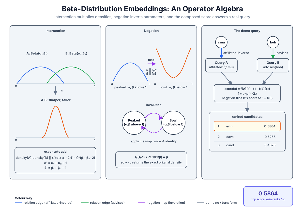The Beta-embedding operator algebra: intersection multiplies densities so exponents add, negation inverts parameters and flips a peaked density into a bowl (an exact involution), and the composed score answers the negation query with erin first. Original diagram by the authors, created with AI assistance.

Training: one-hop queries, manual gradients

The operators are fixed formulas; what training must learn is where the entities sit and what the relations do. Each of the 10 relations (the 5 base relations of the academic graph plus 5 inverses, so a query can walk an edge backwards; beta.py lines 38–40) is an affine map on log-parameters: a learned matrix $W_r \in \mathbb{R}^{2K \times 2K}$ (an 8-by-8 grid of numbers) and a learned shift vector $\mathbf{c}_r \in \mathbb{R}^8$, applied to a head entity's log-parameter vector $\mathbf{p}$ to produce the query's log-parameters

$$\mathbf{q} \;=\; W_r\, \mathbf{p} + \mathbf{c}_r ,$$

implemented in project (beta.py lines 133–135), with $W_r$ initialized near the identity matrix (beta.py lines 121–125). The full parameter ledger is small: 13 entities of 8 numbers (104), plus 10 relations of $64 + 8 = 72$ numbers (720), for 824 trainable parameters in all.

The training data are the 30 one-hop queries built from the 15 training triples of kg.py, each used forwards, "$(h, r, ?)$ should answer $t$", and backwards through the inverse relation (beta.py lines 43–46). The loss for one query is a margin ranking loss on the KL divergence: the true answer $t$ should fit the query at least a margin $\gamma = 1$ better than a uniformly sampled false answer $n$ (resampled while it collides with any known-true triple),

$$L \;=\; \max\!\big(0,\; \gamma + \mathrm{KL}_{\text{pos}} - \mathrm{KL}_{\text{neg}}\big),$$

where $\mathrm{KL}_{\text{pos}} = \mathrm{KL}(\text{entity } t \,\|\, \text{query})$ and $\mathrm{KL}_{\text{neg}}$ is the same for $n$ (beta.py lines 185–211). When the hinge is active, its gradient is $+\partial \mathrm{KL}_{\text{pos}} - \partial \mathrm{KL}_{\text{neg}}$ on every parameter each term touches.

The gradients are written by hand, and they reward the derivation. Differentiate the boxed closed form with respect to $\alpha_1$ (the entity-side parameter). Three terms depend on it; the $\ln B$ term differentiates to a difference of digammas, and the product rule on the two $\psi$ terms gives

$$\frac{\partial}{\partial \alpha_1}\big[-\ln B(\alpha_1, \beta_1)\big] = -\psi(\alpha_1) + \psi(\alpha_1 + \beta_1),$$ $$\frac{\partial}{\partial \alpha_1}\big[(\alpha_1 - \alpha_2)\,\psi(\alpha_1)\big] = \psi(\alpha_1) + (\alpha_1 - \alpha_2)\,\psi'(\alpha_1),$$ $$\frac{\partial}{\partial \alpha_1}\big[(\alpha_2 - \alpha_1 + \beta_2 - \beta_1)\,\psi(\alpha_1 + \beta_1)\big] = -\psi(\alpha_1 + \beta_1) + (\alpha_2 - \alpha_1 + \beta_2 - \beta_1)\,\psi'(\alpha_1 + \beta_1),$$

using $\frac{\partial}{\partial \alpha_1} \ln B(\alpha_1,\beta_1) = \psi(\alpha_1) - \psi(\alpha_1+\beta_1)$ from the KL derivation. Add the three lines: $-\psi(\alpha_1)$ cancels $+\psi(\alpha_1)$, and $+\psi(\alpha_1+\beta_1)$ cancels $-\psi(\alpha_1+\beta_1)$, leaving only derivative-of-digamma terms,

$$\frac{\partial \mathrm{KL}}{\partial \alpha_1} \;=\; (\alpha_1 - \alpha_2)\,\psi'(\alpha_1) \,+\, (\alpha_2 - \alpha_1 + \beta_2 - \beta_1)\,\psi'(\alpha_1 + \beta_1),$$

where $\psi'$ is the trigamma function. The query-side partial is even simpler. The parameter $\alpha_2$ appears in three terms of the boxed formula, and each differentiates in one line, with no product rule surviving, because the $\psi$ factors that $\alpha_2$ multiplies, $\psi(\alpha_1)$ and $\psi(\alpha_1 + \beta_1)$, are constants with respect to $\alpha_2$:

$$\frac{\partial}{\partial \alpha_2}\,\ln B(\alpha_2, \beta_2) \;=\; \psi(\alpha_2) - \psi(\alpha_2 + \beta_2),$$ $$\frac{\partial}{\partial \alpha_2}\big[(\alpha_1 - \alpha_2)\,\psi(\alpha_1)\big] \;=\; -\psi(\alpha_1),$$ $$\frac{\partial}{\partial \alpha_2}\big[(\alpha_2 - \alpha_1 + \beta_2 - \beta_1)\,\psi(\alpha_1 + \beta_1)\big] \;=\; +\psi(\alpha_1 + \beta_1).$$

Summing the three lines, no trigamma survives:

$$\frac{\partial \mathrm{KL}}{\partial \alpha_2} \;=\; \psi(\alpha_2) - \psi(\alpha_2 + \beta_2) - \psi(\alpha_1) + \psi(\alpha_1 + \beta_1).$$

The $\beta$ partials are the mirror images. All four are kl_grads line for line (beta.py lines 100–115). Two chain-rule links then carry these density-space gradients to the actual trainable numbers (beta.py lines 171–182). Through the exponential of the log-parameterization, $\alpha = e^{\ln\alpha}$ gives $\frac{\partial \mathrm{KL}}{\partial \ln\alpha} = \alpha \cdot \frac{\partial \mathrm{KL}}{\partial \alpha}$ (the code's ga1 * a1); and through the affine map $\mathbf{q} = W_r \mathbf{p} + \mathbf{c}_r$, a gradient $\boldsymbol{\delta}_q$ at the query pulls back as

$$\boldsymbol{\delta}_p = W_r^{\top} \boldsymbol{\delta}_q, \qquad \Delta W_r = \boldsymbol{\delta}_q\, \mathbf{p}^{\top}, \qquad \Delta \mathbf{c}_r = \boldsymbol{\delta}_q ,$$

where $W_r^{\top}$ is the transpose (rows and columns exchanged) and $\boldsymbol{\delta}_q \mathbf{p}^{\top}$ is the outer product, the matrix whose $(i,j)$ entry is $\delta_{q,i}\, p_j$. Stochastic gradient descent with step size 0.02 runs 2000 epochs over the 30 queries (beta.py lines 33–35). The committed loss trace shows the hinge emptying out:

training: mean active margin loss  L = max(0, γ + KL_pos − KL_neg)
  epoch     1 :  1.0078
  epoch   100 :  0.0193
  epoch   500 :  0.0000
  epoch  1000 :  0.0000
  epoch  2000 :  0.0000

filtered link prediction (6 queries):  MRR 0.5794  Hits@1 0.3333  Hits@3 0.8333  ranks [3, 7, 1, 1, 2, 2]

By epoch 500 every training query beats every sampled corruption by the full margin. The second line is the shared scoreboard of this volume, kg.evaluate (kg.py lines 110–122), run on the score $s(h, r, t) = -\mathrm{KL}$ over the six filtered ranking queries built from the three held-out triples: a Mean Reciprocal Rank of 0.5794, with four of the six true answers ranked in the top 2. Zero training loss with imperfect test MRR is the usual, honest gap between memorization and generalization on 15 triples; what matters next is that one of those held-out facts is about to be recovered by the geometry inside a harder query.

Composing at the score level, and why

BetaE composes multi-hop queries at the parameter level: it intersects by attention-weighting $(\alpha, \beta)$ vectors and negates with the involution, producing one final Beta vector that is compared to each candidate entity [1]. That works because BetaE is trained end-to-end on multihop query structures: during training, gradients flow through the intersection and negation operators themselves, so the entity embeddings are shaped to make parameter arithmetic meaningful. Our companion model is trained on one-hop queries only, and pretending otherwise would be dishonest. So for composition it drops down one level, from parameters to scores, and says so in its own comment (beta.py lines 157–166):

def and_not(t: int, q_pos: np.ndarray, q_neg: np.ndarray) -> float:
    """Score of the query  q_pos ⊓ ¬q_neg  for entity t, composed at the
    SCORE level with the product t-norm and the standard fuzzy complement:
        f(t) = membership(t, q_pos) · (1 − membership(t, q_neg)).
    BetaE itself composes at the PARAMETER level (attention-weighted sums of
    (α, β), with the involution ``negate`` above), which works when entities
    are trained end-to-end on multihop query structures; with this suite's
    1-hop-only training the score-level composition is the honest,
    well-behaved reading (it is also how CQD composes 1-hop predictors)."""
    return membership(t, q_pos) * (1.0 - membership(t, q_neg))

The ingredients are a small fuzzy logic. membership (beta.py lines 151–154) squashes the divergence into a graded truth value $f(t) = e^{-\mathrm{KL}(t \,\|\, q)}$, which lies in the half-open interval $(0, 1]$ and equals 1 exactly when the entity's four densities coincide with the query's. Conjunction is the product t-norm (t for triangular, the name of the fuzzy-logic family of conjunction operators): multiply the truth values. Negation is the standard fuzzy complement, $1 - f$. Composing calibrated one-hop scores with t-norms rather than training a multihop machine is itself a respectable design, not a concession: it is how CQD (Continuous Query Decomposition) answers complex queries with a pretrained one-hop model [5], and FuzzQE builds its entire query answerer on exactly this connective set, with theory about which t-norms behave [4]. The landscape survey catalogues both composition styles side by side [2]. What the score level costs us is the single reusable query embedding: the answer is a score per entity, not a new object we could feed into yet another operator.

The centerpiece: affiliated⁻(cmu) ⊓ ¬advises(bob)

Now the query this chapter has been building toward, in the notation of Volume 2: $\text{affiliated}^{-}(\text{cmu}) \sqcap \neg\,\text{advises}(\text{bob})$, read "entities affiliated with cmu, minus entities advised by bob." Because the academic world is tiny, the closed-world ground truth can be computed symbolically by scanning all 18 triples (beta.py lines 229–231): the entities affiliated with cmu are $\{\text{carol}, \text{dave}, \text{erin}\}$, the entities bob advises are $\{\text{carol}, \text{dave}\}$, and the set difference leaves exactly $\{\text{erin}\}$. One subtlety makes this a real test rather than a lookup: the triple (erin, affiliated, cmu) is one of the three held-out test triples (kg.py lines 65–69). The model has never seen erin's affiliation as a positive, and, because this suite's negative sampler filters its corruptions against all 18 triples including the held-out ones (beta.py lines 47–49), the fact was never presented as a negative either. Be clear that this filtering is a deliberate choice, not the standard one: the usual "filtered" protocol governs evaluation-time ranking (which kg.py implements), whereas checking training-time corruptions against held-out triples is a mild use of test information that standard knowledge-graph-embedding training does not make. What it buys is a clean reading of the experiment: the signal about erin's affiliation is genuine silence rather than denial, so ranking her first is generalization from the trained geometry, not memorization.

The learned side builds the two operand queries by projection, $q_A = \text{project}(\text{cmu}, \text{affiliated\_inv})$ and $q_B = \text{project}(\text{bob}, \text{advises})$, then ranks all 13 entities by the composed score (beta.py lines 232–237). The committed output:

negation query: affiliated_inv(cmu) ⊓ ¬ advises(bob)
  closed-world ground truth: affiliated_inv(cmu) = ['carol', 'dave', 'erin'] minus advises(bob) = ['carol', 'dave']  →  ['erin']
  top-3 by the composed score f_A · (1 − f_B),  f = exp(−KL):
    entity       KL_A     KL_B    score
    1. erin     0.3925   2.0269   0.5864  * gold
    2. dave     0.5663   2.6270   0.5266
    3. carol    0.1868   0.6634   0.4023

Trace erin's score by hand from the two divergences: $f_A = e^{-0.3925} = 0.6754$ (a good fit to "affiliated with cmu", even though her affiliation was never trained on), $f_B = e^{-2.0269} = 0.1317$ (a poor fit to "advised by bob", correctly), so the composed score is $0.6754 \times (1 - 0.1317) = 0.6754 \times 0.8683 = 0.5864$, the printed number. The full arithmetic for all three:

rank	entity	$\mathrm{KL}_A$	$f_A = e^{-\mathrm{KL}_A}$	$\mathrm{KL}_B$	$1 - f_B$	score $f_A(1 - f_B)$	symbolic verdict
1	erin	0.3925	0.6754	2.0269	0.8683	0.5864	gold: the answer
2	dave	0.5663	0.5676	2.6270	0.9277	0.5266	excluded (bob advises him)
3	carol	0.1868	0.8296	0.6634	0.4849	0.4023	excluded (bob advises her)

Erin ranks first, and the module asserts it, along with the symbolic gold set, before any result is printed (beta.py lines 244–246). But read the near-miss honestly, because it teaches more than the win. Carol is handled beautifully: her advises edge from bob is a training triple, so the model firmly believes it ($\mathrm{KL}_B = 0.6634$ is small, so the complement $1 - f_B = 0.4849$ cuts her score nearly in half). Dave is the interesting case: the triple (bob, advises, dave) is also held out in the test split. The model only weakly suspects it ($\mathrm{KL}_B = 2.6270$, the largest in the table), so the negation barely dents him, and he finishes a close second at 0.5266, just 0.06 behind the gold answer. Generalization cut both ways in a single query: it promoted erin by inferring her unseen affiliation, and it under-suppressed dave by failing to infer his unseen advising edge. A crisp symbolic engine with the full fact set would never rank dave second; a learned geometry that has genuinely not been shown the fact cannot do better than suspect it. That double edge, inference where the symbols are silent, at the price of certainty everywhere, is the entire trade of Part II in one table.

What probability bought, and what it cost

The purchase is real. Densities gave us the first negation operator in this volume with an exact algebraic law behind it (the involution), a conjunction that stays in the family (exponents add, with the weighted form keeping the parameters legal in every regime), and graded membership for free: erin at 0.5864 versus carol at 0.4023 is a ranking with intermediate degrees, something a hard boundary can only fake. The framework also carries a native notion of uncertainty, since a Beta with small $\alpha + \beta$ is spread out and one with large $\alpha + \beta$ is concentrated; BetaE reads the differential entropy of a query's density as the model's uncertainty about it [1].

Here is what was not purchased: calibration. The membership value $f = e^{-\mathrm{KL}}$ lives in $(0, 1]$ and multiplies pleasantly, but nothing in the training objective makes 0.5864 mean "a 58.64 percent chance that erin answers the query." The margin loss only pushed true answers a fixed distance below false ones in divergence; the absolute scores are shaped by $\gamma$, the learning rate, and the initialization, not by any frequency in the world. These are learned scores wearing the costume of probabilities, and the costume is convincing enough to be dangerous. The same caution applies to BetaE itself and to every probabilistic query embedding: the probability calculus is being used as a representation algebra, chosen for its closure properties, not as a calibrated posterior over answers. Whether, and how, such scores can be made to mean their numbers, calibration curves, proper scoring rules, conformal guarantees, is a Volume 5 question, and we flag the debt now so no reader mistakes elegant algebra for measured belief.

The unsolved part

The negation operator is exact as algebra, but what is it as logic? The involution $(\alpha, \beta) \mapsto (1/\alpha, 1/\beta)$ satisfies double negation elimination by construction, and it demonstrably flips high density to low density. What no one has proved is that it implements the set complement of a query's answers under any precise semantics: there is no theorem stating that if entity $t$ answers $q$ with membership $f$, it answers $\neg q$ with anything in particular. The operator was chosen because it has the right symmetries and it trains well, and the same is true of the attention-weighted intersection, which only approximates the density product it is motivated by. Contrast this with Volume 2, where the completion rules came with soundness and completeness theorems tying every derived fact to model theory. The probabilistic query embeddings have closure and differentiability, but as of the current landscape no negation-capable query embedding carries a soundness guarantee connecting its operator algebra to first-order semantics [2]. A second, more local honesty: this chapter's model composes at the score level precisely because parameter-level composition without end-to-end multihop training is unvalidated; the algebra exists, but on this training diet nothing certifies it. Making learned operators provably mean their logical names is an open problem, and it is one of the central demands Volume 4 will place on the neuro-symbolic bridge.

Why it matters

For the arc of this series, this chapter is the moment the neural side first fields a complete set of Boolean connectives. Conjunction (Chapter 5) plus a well-behaved negation yields, in principle, the full propositional repertoire over query embeddings, which is the raw material Volume 4 needs when it starts compiling logic into differentiable objectives: semantic loss, t-norm relaxations, and weighted model counting all presuppose soft connectives with trustworthy algebraic laws, and the product t-norm with complement $1 - f$ used by and_not is exactly the vocabulary those chapters will formalize [4]. The involution is also a small, perfect specimen of a theme the frontier volume will enlarge: a logical law (double negation elimination) holding in a learned system exactly, by architectural construction, rather than approximately, by training. Where laws can be built in, they never need to be learned, and never fail. Finally, the calibration caveat above is the first appearance of the trust question that Volume 5 is entirely about: a system that answers with confident-looking numbers must eventually say what its numbers mean.

Key terms

• Beta distribution — the two-parameter probability density $p(x; \alpha, \beta) = x^{\alpha-1}(1-x)^{\beta-1}/B(\alpha,\beta)$ on the unit interval; each entity and query here is a vector of $K = 4$ of them.
• Shape parameters $\alpha, \beta$ — the exponents-plus-one of the density; each parameter above 1 pushes mass away from its end of the interval, below 1 piles mass onto it.
• Log-parameterization — storing $(\ln\alpha, \ln\beta)$ so gradient descent moves in $\mathbb{R}^{2K}$ while the parameters stay positive; it turns negation into a sign flip.
• KL divergence (Beta closed form) — $\ln B_2 - \ln B_1 + (\alpha_1{-}\alpha_2)\psi(\alpha_1) + (\beta_1{-}\beta_2)\psi(\beta_1) + (\alpha_2{-}\alpha_1{+}\beta_2{-}\beta_1)\psi(\alpha_1{+}\beta_1)$, summed over components; the fit measure of the whole model.
• Digamma / trigamma — $\psi = (\ln\Gamma)'$ and $\psi'$; computed from scratch by the recurrence $\psi(x+1) = \psi(x) + 1/x$ plus an asymptotic series, self-checked to $10^{-12}$.
• Involution — a map that is its own inverse; BetaE's negation $(\alpha, \beta) \mapsto (1/\alpha, 1/\beta)$ is one, so double negation is exactly the identity.
• Product t-norm / fuzzy complement — the score-level connectives $f_1 \cdot f_2$ and $1 - f$ used by and_not on the graded membership $f = e^{-\mathrm{KL}}$.
• EPFO — the existential positive first-order query fragment ($\exists, \wedge, \vee$); regions handle it, and negation is precisely what lies beyond it.
• Closure under complement — the property boxes and balls lack (their complements are unbounded and leave the family) and densities supply.
• Calibration — the missing guarantee: a score of 0.5864 is a learned ranking value, not a 58.64 percent probability.

Where this leads

Part II now holds three competing geometries: balls placed by hand, boxes trained on paths, and densities that can negate. Before the Part closes, the first two must settle an old score. Chapter 4 claimed, in passing, that the intersection of two balls is a lens and a lens is not a ball; Chapter 5 built an empire on the box's closure under intersection. The next chapter, Boxes versus Balls, turns that passing claim into a measured verdict: it derives the smallest enclosing ball of a lens in three lines of algebra, exhibits a provable false positive by coordinates, and measures the false-positive area on a dense grid, no training and no loss, just geometry deciding which family deserves the ontology-embedding chapters of Part III.

---

Companion code: examples/neural/beta.py implements everything in this chapter with no dependency beyond NumPy: the from-scratch digamma and trigamma, the closed-form Beta KL and its four hand-derived partials, the sign-flip negation with its $10^{-12}$ double-negation check, the margin-loss training loop, and the negation query with its symbolic ground truth asserted before any result prints. Run python3 examples/neural/beta.py (seeded, deterministic) to reproduce every number quoted above; examples/neural/kg.py supplies the 18 triples, the 15/3 split, and the shared filtered-ranking evaluation.