Balls and Cones: Concepts as Regions

📍 Where we are: Part II · Region and Geometric Embeddings — Chapter 4. Bilinear Models closed Part I with entities as points and relations as multiplicative interactions between them; this chapter opens Part II by proving what a symmetric comparison of points can never do, and giving concepts the geometry they actually want.

Part I embedded the academic world's individuals: alice, bob, and p1 became vectors, and relations became operations that score pairs of vectors. But the academic world contains a second kind of object that Part I never touched. Professor, Researcher, and Student are concepts, and a concept denotes a set of individuals. Volume 2 reasoned about the relations between those sets: Professor ⊑ Researcher says one set sits inside another; Professor ⊓ Student ⊑ ⊥ says two sets share nothing. Can geometry carry that structure? The first answer is negative: any comparison of two points by a distance or a dot product returns the same number in both directions, and a symmetric score cannot carry set inclusion, which holds one way and fails the other. The fix is to let a concept be a region of the space. Membership, subsumption, and disjointness then each become one closed-form geometric test, and we will build a concrete geometry in which all three agree exactly with the symbolic gold standard.

The simple version

Imagine a wall map of a campus. You could mark "the Physics Department" with a pin, the way Part I pinned alice. But a department is not a spot; it is an area. Draw it as a fenced region instead and questions no pin can answer become a glance: is this person inside the fence (membership)? Does this fence sit entirely inside the Science Quad's fence (that is what "every physicist is a scientist" looks like)? Do two fences overlap at all (disjointness)? A pin can only be near another pin, and "near" works both ways; a fence can contain another fence, and containment works one way only. Concepts are fences, not pins. This chapter draws the fences by hand and checks that they agree with everything Volume 2 proved.

What this chapter covers

• Why symmetrically scored points fail concepts: subsumption is set inclusion, asymmetric and transitive; distances and dot products are symmetric, and we derive the mismatch rather than assert it.
• The ball, formally: a concept as a center and a radius; membership as $\lVert \mathbf{x} - \mathbf{c} \rVert \le r$, decoded symbol by symbol.
• The containment theorem, proved both ways: ball(c₁, r₁) sits inside ball(c₂, r₂) if and only if $\lVert \mathbf{c}_1 - \mathbf{c}_2 \rVert + r_1 \le r_2$; the triangle inequality does one direction, a "worst point" construction the other; disjointness likewise.
• The academic geometry, placed by hand: eight balls and thirteen points from regions.py, verified against Volume 2's classification: 8 of 8 gold subsumptions, 0 spurious among 56 ordered pairs, 7 of 7 separations, 13 of 13 membership sets.
• Transitivity for free: composing two containment inequalities yields the third; geometry inherits the logic's structure when the construction is faithful.
• Cones and order embeddings: is-a as a coordinatewise inequality under the reversed product order, transitive pairs derived rather than asserted, and (Paper, Person) genuinely incomparable.
• What construction proves and training must earn: this chapter places regions to show the geometry is expressive enough; Part III must learn them, and soundness drops from guarantee to probe.
• The unsolved part: one radius makes concepts isotropic, and the intersection of two balls is not a ball: the flaws the next chapter's boxes repair.

Why symmetrically scored points fail concepts

Start with what Part I gives us. An entity is a vector $\mathbf{e} \in \mathbb{R}^n$, where $\mathbb{R}^n$ is the space of lists of $n$ real numbers and $n$ is the embedding dimension. A score function compares two such vectors: TransE by a distance, the norm $\lVert \mathbf{e}_h + \mathbf{w}_r - \mathbf{e}_t \rVert$, where the norm $\lVert \mathbf{v} \rVert$ of a vector is its length, the square root of the sum of its squared coordinates, so that $\lVert \mathbf{v} \rVert^2 = \sum_{j=1}^{n} v_j^2$ with $v_j$ the $j$-th coordinate; DistMult by a weighted dot product. Suppose we reuse this machinery for concepts: give Professor a vector $\mathbf{e}_P$, give Researcher a vector $\mathbf{e}_R$, and read Professor ⊑ Researcher off some comparison $s(\mathbf{e}_P, \mathbf{e}_R)$.

Here is the obstruction, derived. Subsumption is set inclusion: $C \sqsubseteq D$ means every member of $C$ is a member of $D$; for plain sets the same relation is written $C \subseteq D$, read "$C$ is a subset of $D$" (the square symbol $\sqsubseteq$ is reserved for concepts). Inclusion is a partial order: reflexive (every set includes itself), transitive (if $C \subseteq D$ and $D \subseteq E$ then $C \subseteq E$), and antisymmetric, holding in at most one direction for distinct sets (two concept names that subsume each other denote the same set; Volume 2's classification treats such names as equivalent). Professor ⊑ Researcher is true and Researcher ⊑ Professor is false, and a representation of subsumption must be able to say so. Now compute what the two standard comparisons say about an ordered pair taken in both orders. For distance, write the difference vector $\mathbf{v} = \mathbf{e}_P - \mathbf{e}_R$ and expand the squared norm of its negation coordinate by coordinate:

$$\lVert -\mathbf{v} \rVert^2 \;=\; \sum_{j=1}^{n} (-v_j)^2 \;=\; \sum_{j=1}^{n} v_j^2 \;=\; \lVert \mathbf{v} \rVert^2,$$

so $\lVert \mathbf{e}_P - \mathbf{e}_R \rVert = \lVert \mathbf{e}_R - \mathbf{e}_P \rVert$: the distance from Professor to Researcher equals the distance back, for every possible placement of the two points. For the dot product the same symmetry falls out of the commutativity of multiplication:

$$\mathbf{e}_P \cdot \mathbf{e}_R \;=\; \sum_{j=1}^{n} e_{P,j}\, e_{R,j} \;=\; \sum_{j=1}^{n} e_{R,j}\, e_{P,j} \;=\; \mathbf{e}_R \cdot \mathbf{e}_P.$$

Any score built from either quantity therefore assigns the true statement Professor ⊑ Researcher and its false converse exactly the same number; no threshold can accept one and reject the other. Asymmetric point scores do exist: ComplEx escaped this trap for facts by scoring ordered triples through a complex conjugation, and a relation-parameterized comparison such as TransE's translated distance is not symmetric either: with the difference vector $\mathbf{v} = \mathbf{e}_P - \mathbf{e}_R$ from above, the two directions score $\lVert \mathbf{e}_P + \mathbf{w}_r - \mathbf{e}_R \rVert = \lVert \mathbf{v} + \mathbf{w}_r \rVert$ and $\lVert \mathbf{e}_R + \mathbf{w}_r - \mathbf{e}_P \rVert = \lVert \mathbf{w}_r - \mathbf{v} \rVert$, expanding both squared norms gives $\lVert \mathbf{v} + \mathbf{w}_r \rVert^2 = \lVert \mathbf{v} \rVert^2 + 2\, \mathbf{w}_r \cdot \mathbf{v} + \lVert \mathbf{w}_r \rVert^2$ and $\lVert \mathbf{w}_r - \mathbf{v} \rVert^2 = \lVert \mathbf{w}_r \rVert^2 - 2\, \mathbf{w}_r \cdot \mathbf{v} + \lVert \mathbf{v} \rVert^2$, so the two scores differ exactly when the dot product $\mathbf{w}_r \cdot \mathbf{v}$ is nonzero, which a generic placement satisfies (they coincide in the special case where $\mathbf{w}_r$ is perpendicular to $\mathbf{v}$). But these escapes are pointwise: the model can learn to prefer one asserted pair over its reverse, yet nothing forces transitivity, and nothing gives a membership semantics. The lexical-semantics literature reached the same diagnosis early: a word's meaning has an extension, an inside and an outside, and a single point has neither [1].

So we change the ontology of the embedding space itself. Keep individuals as points, because an individual is one thing. Make each concept a region, a subset $\mathrm{reg}(C) \subseteq \mathbb{R}^n$, because a concept is a set of things. The three judgments of Volume 2 then translate structurally, not just trainably:

logical judgment	Volume 2 reading	geometric test
membership $a : C$	the individual $a$ is an instance of $C$	point $\mathbf{x}_a$ lies inside $\mathrm{reg}(C)$
subsumption $C \sqsubseteq D$	every $C$ is a $D$	$\mathrm{reg}(C) \subseteq \mathrm{reg}(D)$
disjointness $C \sqcap D \sqsubseteq \bot$	nothing is both	$\mathrm{reg}(C) \cap \mathrm{reg}(D) = \varnothing$

Region containment is reflexive, transitive, and antisymmetric because set inclusion is; the asymmetry we could not buy with points comes free with regions. What remains is to pick a family of regions simple enough that all three tests have closed forms. The simplest candidate is the ball.

The ball: one center, one radius, three closed-form tests

Fix the ambient space $\mathbb{R}^n$; in this chapter $n = 2$, so every construction can be drawn and every number checked by hand. A ball is determined by two parameters: a center $\mathbf{c} \in \mathbb{R}^n$, the point the concept sits around, and a radius $r \ge 0$, how far it reaches. The ball is the set of points within distance $r$ of the center:

$$B(\mathbf{c}, r) \;=\; \{\, \mathbf{x} \in \mathbb{R}^n \;:\; \lVert \mathbf{x} - \mathbf{c} \rVert \le r \,\}.$$

The norm $\lVert \cdot \rVert$ was decoded in the opening section (the Euclidean length, the square root of the sum of the squared coordinates), so $\lVert \mathbf{x} - \mathbf{c} \rVert$ is the straight-line distance between the point $\mathbf{x}$ and the center $\mathbf{c}$. The inequality is non-strict, so the ball is closed: it includes its boundary circle. Membership is a single comparison, implemented in one line (regions.py lines 72–76):

def in_ball(p: Point, concept: str) -> bool:
    """Membership: x ∈ ball(c, r)  ⟺  ‖x − c‖ ≤ r."""
    c, r = BALLS[concept]
    # membership test:  ‖x − c‖ ≤ r
    return dist(p, c) <= r

Everything else in this chapter rests on one theorem of the geometry, the triangle inequality: for any two vectors $\mathbf{u}$ and $\mathbf{v}$,

$$\lVert \mathbf{u} + \mathbf{v} \rVert \;\le\; \lVert \mathbf{u} \rVert + \lVert \mathbf{v} \rVert,$$

a detour through a corner is never shorter than the straight line. We use it in its three-point form: for any points $\mathbf{x}, \mathbf{y}, \mathbf{z}$, substitute $\mathbf{u} = \mathbf{x} - \mathbf{y}$ and $\mathbf{v} = \mathbf{y} - \mathbf{z}$, so that $\mathbf{u} + \mathbf{v} = \mathbf{x} - \mathbf{y} + \mathbf{y} - \mathbf{z} = \mathbf{x} - \mathbf{z}$, and the inequality becomes

$$\lVert \mathbf{x} - \mathbf{z} \rVert \;\le\; \lVert \mathbf{x} - \mathbf{y} \rVert + \lVert \mathbf{y} - \mathbf{z} \rVert :$$

the distance from $\mathbf{x}$ to $\mathbf{z}$ is at most the distance via any waypoint $\mathbf{y}$. This one fact proves containment, disjointness, and transitivity below.

The containment theorem, proved in both directions

Here is the claim that makes balls usable as concepts: containment of one ball in another, a statement quantified over infinitely many points, collapses to one comparison of three numbers.

Theorem. For balls with centers $\mathbf{c}_1, \mathbf{c}_2$ and radii $r_1, r_2$:

$$B(\mathbf{c}_1, r_1) \subseteq B(\mathbf{c}_2, r_2) \quad\Longleftrightarrow\quad \lVert \mathbf{c}_1 - \mathbf{c}_2 \rVert + r_1 \;\le\; r_2.$$

In words: the inner ball fits inside the outer one exactly when the distance between the centers, plus the inner radius, still fits inside the outer radius. Both directions deserve proof, because each does a different job. The (⇐) direction makes the test sound: if the inequality holds, containment really holds. The (⇒) direction makes the test exact: if the inequality fails, containment really fails.

Direction (⇐): the inequality forces containment. Assume $\lVert \mathbf{c}_1 - \mathbf{c}_2 \rVert + r_1 \le r_2$, and take an arbitrary point $\mathbf{x}$ of the inner ball, so $\lVert \mathbf{x} - \mathbf{c}_1 \rVert \le r_1$. We must show $\lVert \mathbf{x} - \mathbf{c}_2 \rVert \le r_2$. Route the distance from $\mathbf{x}$ to $\mathbf{c}_2$ through the waypoint $\mathbf{c}_1$ and chain three inequalities, each justified as it is used:

$$\lVert \mathbf{x} - \mathbf{c}_2 \rVert \;\underset{\text{triangle}}{\le}\; \lVert \mathbf{x} - \mathbf{c}_1 \rVert + \lVert \mathbf{c}_1 - \mathbf{c}_2 \rVert \;\underset{\mathbf{x}\, \in\, \text{inner}}{\le}\; r_1 + \lVert \mathbf{c}_1 - \mathbf{c}_2 \rVert \;\underset{\text{assumption}}{\le}\; r_2 .$$

The point $\mathbf{x}$ was arbitrary, so every point of the inner ball lies in the outer ball: the triangle inequality handled all infinitely many members at once.

Direction (⇒): if the inequality fails, a witness escapes. Now assume $\lVert \mathbf{c}_1 - \mathbf{c}_2 \rVert + r_1 \gt r_2$, and exhibit a point of the inner ball lying outside the outer one. The right witness is the worst point of the inner ball: the point of $B(\mathbf{c}_1, r_1)$ farthest from $\mathbf{c}_2$. Geometrically, stand at $\mathbf{c}_2$, look toward $\mathbf{c}_1$, and keep walking past $\mathbf{c}_1$ for $r_1$ more. Formally, suppose first $\mathbf{c}_1 \neq \mathbf{c}_2$ and let

$$\mathbf{u} \;=\; \frac{\mathbf{c}_1 - \mathbf{c}_2}{\lVert \mathbf{c}_1 - \mathbf{c}_2 \rVert}, \qquad \mathbf{w} \;=\; \mathbf{c}_1 + r_1\, \mathbf{u}.$$

Here $\mathbf{u}$ is the unit vector (length one, because we divided the difference by its own norm) pointing from $\mathbf{c}_2$ toward $\mathbf{c}_1$, and $\mathbf{w}$ continues from $\mathbf{c}_1$ in that outward direction for distance $r_1$. First, $\mathbf{w}$ belongs to the inner ball, with no slack:

$$\lVert \mathbf{w} - \mathbf{c}_1 \rVert \;=\; \lVert r_1 \mathbf{u} \rVert \;=\; r_1 \lVert \mathbf{u} \rVert \;=\; r_1 .$$

Second, compute its distance to $\mathbf{c}_2$. Since $\mathbf{c}_1 - \mathbf{c}_2 = \lVert \mathbf{c}_1 - \mathbf{c}_2 \rVert\, \mathbf{u}$ by the definition of $\mathbf{u}$, the two segments point the same way and their lengths add exactly:

$$\mathbf{w} - \mathbf{c}_2 \;=\; (\mathbf{c}_1 - \mathbf{c}_2) + r_1 \mathbf{u} \;=\; \big( \lVert \mathbf{c}_1 - \mathbf{c}_2 \rVert + r_1 \big)\, \mathbf{u},$$ $$\lVert \mathbf{w} - \mathbf{c}_2 \rVert \;=\; \big( \lVert \mathbf{c}_1 - \mathbf{c}_2 \rVert + r_1 \big)\, \lVert \mathbf{u} \rVert \;=\; \lVert \mathbf{c}_1 - \mathbf{c}_2 \rVert + r_1 \;\gt\; r_2 .$$

So $\mathbf{w}$ is a member of the inner ball sitting strictly outside the outer ball, and containment fails. (If instead $\mathbf{c}_1 = \mathbf{c}_2$, the failed inequality reads $r_1 \gt r_2$; pick any unit vector $\mathbf{u}$ and the same $\mathbf{w}$ sits at distance $r_1 \gt r_2$ from $\mathbf{c}_2$.) ∎ (The tombstone symbol ∎ marks the end of a proof.)

The companion implementation is the theorem's right-hand side verbatim, and its docstring is this proof compressed (regions.py lines 79–91):

def ball_subsumed(inner: str, outer: str) -> bool:
    """Containment: ball(c1, r1) ⊆ ball(c2, r2)  ⟺  ‖c1 − c2‖ + r1 ≤ r2.

    (⇐) For any x in the inner ball the triangle inequality gives
    ‖x − c2‖ ≤ ‖x − c1‖ + ‖c1 − c2‖ ≤ r1 + ‖c1 − c2‖ ≤ r2, so x lies in the
    outer ball too.  (⇒, the test is *exact*) the inner ball's farthest point
    from c2 — walk from c1 directly away from c2 for r1 more — sits at
    distance exactly ‖c1 − c2‖ + r1 from c2, so if the inequality fails, that
    point of the inner ball escapes the outer one.
    """
    (c1, r1), (c2, r2) = BALLS[inner], BALLS[outer]
    # containment test:  ‖c1 − c2‖ + r1 ≤ r2
    return dist(c1, c2) + r1 <= r2

Disjointness by the same tool. Two balls are disjoint when no point lies in both, and the triangle inequality again reduces the quantifier to arithmetic. Suppose some $\mathbf{x}$ belonged to both, so $\lVert \mathbf{c}_1 - \mathbf{x} \rVert \le r_1$ and $\lVert \mathbf{x} - \mathbf{c}_2 \rVert \le r_2$. Routing the center-to-center distance through $\mathbf{x}$:

$$\lVert \mathbf{c}_1 - \mathbf{c}_2 \rVert \;\le\; \lVert \mathbf{c}_1 - \mathbf{x} \rVert + \lVert \mathbf{x} - \mathbf{c}_2 \rVert \;\le\; r_1 + r_2 .$$

Contrapositive: if $\lVert \mathbf{c}_1 - \mathbf{c}_2 \rVert \gt r_1 + r_2$, no shared point can exist, and the balls are disjoint. One honest boundary note: at exact equality the closed balls are not quite disjoint; they touch in a single tangent point, where both membership inequalities hold with equality. The companion test uses $\ge$ (regions.py lines 94–104), which is legitimate there because the construction keeps every declared-disjoint pair strictly apart (the tightest pairs, Professor versus Student and Paper versus Topic, sit at center distance 8 against a radius sum of 6). A concept is now two parameters, and each of the three logical judgments is one comparison. Time to build the academic world.

The academic geometry, placed by hand

The companion file examples/neural/regions.py gives the eight concepts of the academic hierarchy explicit centers and radii, chosen as small round numbers so every test below is exact in floating point (regions.py lines 54–63). Nothing is trained, sampled, or seeded; every run prints byte-identical output by construction. The placement, quoted from the real run:

1. the ball system (a concept = center c ∈ ℝ² and radius r)
   concept     | center        | radius
   Person      | (  0.0,  0.0) |   10.0
   Researcher  | (  0.0, -1.0) |    7.0
   Professor   | ( -4.0, -1.0) |    3.0
   Student     | (  4.0, -1.0) |    3.0
   Dean        | ( -5.0, -1.0) |    1.0
   Paper       | ( 20.0,  0.0) |    3.0
   Institution | ( 20.0, -8.0) |    2.0
   Topic       | ( 28.0,  0.0) |    3.0

Read the design off the numbers. Person is the big ball; Researcher sits just inside it; Professor and Student hang symmetrically off Researcher's left and right; Dean nests inside Professor; the three non-person sorts (Paper, Institution, Topic) live far to the right. Radius encodes generality: the more general the concept, the larger its ball, because it must contain the balls of all its specializations.

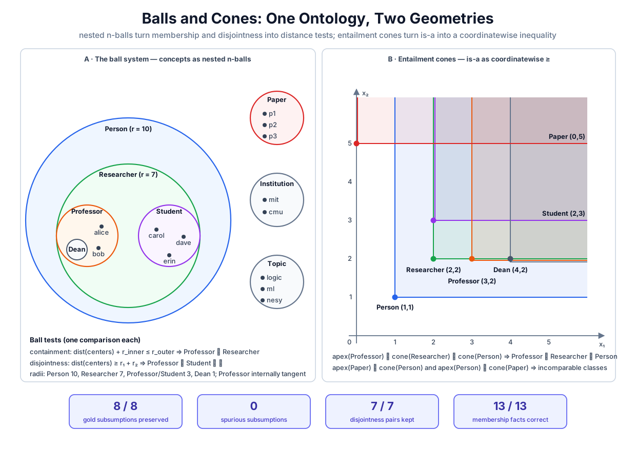Two geometries for one ontology: nested balls make membership, subsumption, and disjointness single comparisons, while order-embedding cones make is-a a coordinatewise inequality; both reproduce Volume 2's eight gold subsumptions exactly. Original diagram by the authors, created with AI assistance.

The gold standard this geometry must reproduce is not typed in by hand: the verification routine asserts that the eight-pair GOLD list equals Volume 2's el_completion.classify() restricted to the eight ball concepts (regions.py lines 111–116 and 203–226), so the scoreboard is checked against the symbolic reasoner itself. The run then applies the containment theorem to all eight gold pairs:

gold subsumption	$\lVert \mathbf{c}_1 - \mathbf{c}_2 \rVert$	$+\, r_1$	total	$\le r_2$?	slack
Dean ⊑ Professor	$1.0000$	$1.0$	$2.0000$	$\le 3.0$ ✓	$1.0000$
Dean ⊑ Researcher	$5.0000$	$1.0$	$6.0000$	$\le 7.0$ ✓	$1.0000$
Dean ⊑ Person	$5.0990$	$1.0$	$6.0990$	$\le 10.0$ ✓	$3.9010$
Professor ⊑ Researcher	$4.0000$	$3.0$	$7.0000$	$\le 7.0$ ✓	$0.0000$
Professor ⊑ Person	$4.1231$	$3.0$	$7.1231$	$\le 10.0$ ✓	$2.8769$
Student ⊑ Researcher	$4.0000$	$3.0$	$7.0000$	$\le 7.0$ ✓	$0.0000$
Student ⊑ Person	$4.1231$	$3.0$	$7.1231$	$\le 10.0$ ✓	$2.8769$
Researcher ⊑ Person	$1.0000$	$7.0$	$8.0000$	$\le 10.0$ ✓	$2.0000$

Two rows deserve a second look. Professor ⊑ Researcher holds with slack exactly zero: $4 + 3 = 7$, a deliberate internal tangency (regions.py lines 51–53). The worst point of the Professor ball as seen from Researcher's center, the point $(-7, -1)$, lies exactly on Researcher's boundary circle, and because both balls are closed, containment still holds. The construction puts the test at its boundary case on purpose: it shows the theorem's $\le$ is the correct comparison, not a convenient approximation, and since every quantity is a small integer the floating-point test is exact.

Holding the eight gold pairs is only half the requirement; a geometry that made everything contain everything would also pass that half. Soundness demands the complement: no containment the logic does not sanction. The run therefore scans all $8 \cdot 7 = 56$ ordered pairs of distinct concepts (regions.py lines 207–210) and prints the incidence matrix:

   full scan of all 8·7 = 56 ordered pairs (A ≠ B): 8 hold — exactly the gold 8, spurious 0
   A ⊆ B?      Pers Rsch Prof Stud Dean Papr Inst Topc
   Person         —    ·    ·    ·    ·    ·    ·    ·
   Researcher     ⊑    —    ·    ·    ·    ·    ·    ·
   Professor      ⊑    ⊑    —    ·    ·    ·    ·    ·
   Student        ⊑    ⊑    ·    —    ·    ·    ·    ·
   Dean           ⊑    ⊑    ⊑    ·    —    ·    ·    ·
   Paper          ·    ·    ·    ·    ·    —    ·    ·
   Institution    ·    ·    ·    ·    ·    ·    —    ·
   Topic          ·    ·    ·    ·    ·    ·    ·    —

Exactly eight cells carry a ⊑, and they are exactly the gold eight: zero spurious containments. The disjointness checks pass with visible margins, the tightest (jointly with Paper versus Topic, both at margin $2$) being the one the TBox axiom Professor ⊓ Student ⊑ ⊥ demands:

3. disjointness — ball(c1,r1) ∩ ball(c2,r2) = ∅  ⟸  ‖c1−c2‖ ≥ r1 + r2
   Professor   vs Student     : ‖c1−c2‖ =  8.0000 ≥ r1 + r2 =  6.0  ✓
   Person      vs Paper       : ‖c1−c2‖ = 20.0000 ≥ r1 + r2 = 13.0  ✓

with the remaining five sort separations (Person against Institution and Topic, and the three pairs among Paper, Institution, Topic) passing the same way (regions.py lines 126–130 and 213).

The thirteen individuals. Every entity of the knowledge graph (kg.py line 49 fixes the entity list, line 58 the type map) gets a point inside its concept's ball (regions.py lines 139–153). The requirement is sharp in both directions: an individual must lie in every ball of its type's reflexive ancestor set and in no other. The run checks all $13 \times 8 = 104$ membership tests:

4. the 13 individuals as points — x ∈ ball(c,r)  ⟺  ‖x−c‖ ≤ r
   entity | type        | point         | member of
   alice  | Professor   | ( -3.0, -1.0) | Person Researcher Professor  ✓
   bob    | Professor   | ( -4.0,  1.0) | Person Researcher Professor  ✓
   carol  | Student     | (  3.0, -1.0) | Person Researcher Student  ✓
   cmu    | Institution | ( 21.0, -8.0) | Institution  ✓
   dave   | Student     | (  5.0, -1.0) | Person Researcher Student  ✓
   erin   | Student     | (  4.0,  0.0) | Person Researcher Student  ✓
   ...
   every individual lies in exactly its ancestors' balls: 13/13

Trace one row by hand. Take bob at $(-4, 1)$, asserted a Professor. Against the Professor ball, center $(-4, -1)$, radius $3$: the difference vector is $(0, 2)$, so $\lVert \mathbf{x} - \mathbf{c} \rVert = \sqrt{0^2 + 2^2} = 2 \le 3$, member. Against Researcher, center $(0, -1)$, radius $7$: difference $(-4, 2)$, distance $\sqrt{16 + 4} = \sqrt{20} \approx 4.4721 \le 7$, member. Against Person, center $(0,0)$, radius $10$: distance $\sqrt{16 + 1} = \sqrt{17} \approx 4.1231 \le 10$, member. Against Dean, center $(-5, -1)$, radius $1$: difference $(1, 2)$, distance $\sqrt{5} \approx 2.2361 \gt 1$, not a member. That exclusion matters: both professors are deliberately placed outside the Dean ball nested within Professor, because nobody in the academic world is asserted to be a dean, and a faithful geometry must not volunteer memberships the knowledge base never licensed. The run's bottom line collects the scoreboard:

SUMMARY regions: gold=8/8 spurious=0 disjoint=7/7 membership=13/13 cone_pairs=8 cone_matches_gold=True

Every count in that line is guarded by an assert (regions.py lines 224–244), so the module's exit code is the acceptance verdict: if any geometric claim in this chapter broke, python3 regions.py would crash rather than print.

Transitivity for free

Volume 2 worked for transitivity: completion rule CR1 fired repeatedly to chain Dean ⊑ Professor and Professor ⊑ Researcher into Dean ⊑ Researcher. The ball geometry gets the same closure without any rule firing, and the reason is an algebraic identity, not a coincidence of this placement.

Suppose the containment test holds for two nested pairs: ball 1 inside ball 2, and ball 2 inside ball 3,

$$\lVert \mathbf{c}_1 - \mathbf{c}_2 \rVert + r_1 \;\le\; r_2, \qquad \lVert \mathbf{c}_2 - \mathbf{c}_3 \rVert + r_2 \;\le\; r_3 .$$

Claim: the test holds for ball 1 inside ball 3. Start from the quantity to be bounded and route the center distance through $\mathbf{c}_2$ by the triangle inequality:

$$\lVert \mathbf{c}_1 - \mathbf{c}_3 \rVert + r_1 \;\le\; \lVert \mathbf{c}_1 - \mathbf{c}_2 \rVert + \lVert \mathbf{c}_2 - \mathbf{c}_3 \rVert + r_1 .$$

Group the first and last terms and apply the first assumption, $\lVert \mathbf{c}_1 - \mathbf{c}_2 \rVert + r_1 \le r_2$:

$$\lVert \mathbf{c}_1 - \mathbf{c}_2 \rVert + r_1 + \lVert \mathbf{c}_2 - \mathbf{c}_3 \rVert \;\le\; r_2 + \lVert \mathbf{c}_2 - \mathbf{c}_3 \rVert .$$

Now apply the second assumption to the right-hand side, $\lVert \mathbf{c}_2 - \mathbf{c}_3 \rVert + r_2 \le r_3$:

$$r_2 + \lVert \mathbf{c}_2 - \mathbf{c}_3 \rVert \;\le\; r_3 .$$

Chaining the three displays gives $\lVert \mathbf{c}_1 - \mathbf{c}_3 \rVert + r_1 \le r_3$, which is the containment test for the outer pair. ∎

Instantiate it on the running example. Dean ⊑ Professor holds with $1 + 1 = 2 \le 3$, and Professor ⊑ Researcher with $4 + 3 = 7 \le 7$; the composition therefore guarantees Dean ⊑ Researcher before anyone measures it, and the direct measurement agrees: $\lVert(-5,-1) - (0,-1)\rVert + 1 = 5 + 1 = 6 \le 7$, with room to spare. That slack is traceable. The three centers are collinear here, so the triangle step in the composition is an equality, $1 + 4 = 5$; all the slack therefore comes from the first premise, Dean ⊑ Professor holding with $2 \le 3$, and that one unit is exactly the gap between the measured $6$ and the guaranteed bound $7$. (With non-collinear centers the triangle step would contribute additional slack of its own.) This is the deeper point of the construction. Subsumption is transitive because set inclusion is; ball containment is transitive because the triangle inequality composes. When the representation's algebra mirrors the logic's structure, inference rules the symbolic side had to execute become theorems the geometric side gets for free: the completion algorithm derived Dean ⊑ Researcher in a saturation pass, while the geometry cannot even represent a state in which it fails while the two premises hold.

Cones: is-a as a coordinatewise inequality

Balls are not the only region family with these properties. Order embeddings deliver the same asymmetry-plus-transitivity package with even less machinery: no radius, no norm, just the ordering of real numbers applied one coordinate at a time [2].

Decode the order first. For two points $\mathbf{x}, \mathbf{y} \in \mathbb{R}^n$, write $\mathbf{x} \ge \mathbf{y}$ coordinatewise to mean $x_k \ge y_k$ for every dimension index $k$ from $1$ to $n$; if some coordinates go one way and some the other, the points are incomparable, neither $\ge$ the other. An order embedding assigns each concept a single point, its apex, and declares

$$x \text{ is-a } y \quad\Longleftrightarrow\quad \mathbf{x} \ge \mathbf{y} \ \text{coordinatewise},$$

the reversed product order: the more specific concept sits at the larger coordinates. The region reading is what earns this a place in this chapter. Define the cone of a concept as everything coordinatewise above its apex,

$$\mathrm{cone}(\mathbf{y}) \;=\; \{\, \mathbf{p} \in \mathbb{R}^n : \mathbf{p} \ge \mathbf{y} \,\},$$

the closed axis-aligned orthant whose corner is the apex. A general concept near the origin owns a huge cone; a specific concept far out owns a small one. The pointwise order and the region order coincide, by a two-line proof. If $\mathbf{x} \ge \mathbf{y}$, take any $\mathbf{p} \in \mathrm{cone}(\mathbf{x})$; then $\mathbf{p} \ge \mathbf{x} \ge \mathbf{y}$, and since $\ge$ is transitive in each coordinate separately, $\mathbf{p} \ge \mathbf{y}$, so $\mathrm{cone}(\mathbf{x}) \subseteq \mathrm{cone}(\mathbf{y})$. Conversely, $\mathbf{x} \ge \mathbf{x}$ puts $\mathbf{x}$ inside its own cone, so $\mathrm{cone}(\mathbf{x}) \subseteq \mathrm{cone}(\mathbf{y})$ forces $\mathbf{x} \in \mathrm{cone}(\mathbf{y})$, which is the statement $\mathbf{x} \ge \mathbf{y}$. Notice how this evades the opening section's obstruction without contradicting it: each concept is again a single point, but the comparison is the coordinatewise order, asymmetric and transitive where distance and dot product were symmetric, and the cone region supplies the membership semantics a bare point lacked. Membership, subsumption, and the region picture collapse into one test, implemented in one line (regions.py lines 178–181):

def cone_isa(x: str, y: str) -> bool:
    """x is-a y  ⟺  x ≥ y in every coordinate (the reversed product order)."""
    # coordinatewise order test:  CONE[x][k] ≥ CONE[y][k] for every dimension k
    return bool(np.all(np.asarray(CONE[x]) >= np.asarray(CONE[y])))

The companion file places six apexes by hand (regions.py lines 168–175) and then scans all $6 \cdot 5 = 30$ ordered pairs rather than asserting any is-a link directly. The real run:

5. entailment cones — x is-a y  ⟺  x ≥ y coordinatewise (reversed product order)
   concept     | apex   | region
   Person      | (1, 1) | cone(Person) = {p : p ≥ (1, 1)}
   Researcher  | (2, 2) | cone(Researcher) = {p : p ≥ (2, 2)}
   Professor   | (3, 2) | cone(Professor) = {p : p ≥ (3, 2)}
   Student     | (2, 3) | cone(Student) = {p : p ≥ (2, 3)}
   Dean        | (4, 2) | cone(Dean) = {p : p ≥ (4, 2)}
   Paper       | (0, 5) | cone(Paper) = {p : p ≥ (0, 5)}
   derived is-a pairs (scan of all 6·5 = 30 ordered pairs): 8
     Dean       is-a Person     : (4, 2) ≥ (1, 1)
     Dean       is-a Professor  : (4, 2) ≥ (3, 2)
     Dean       is-a Researcher : (4, 2) ≥ (2, 2)
     Professor  is-a Person     : (3, 2) ≥ (1, 1)
     Professor  is-a Researcher : (3, 2) ≥ (2, 2)
     Researcher is-a Person     : (2, 2) ≥ (1, 1)
     Student    is-a Person     : (2, 3) ≥ (1, 1)
     Student    is-a Researcher : (2, 3) ≥ (2, 2)
   transitivity is inherited from ≥ : Professor(3,2) ≥ Researcher(2,2) ≥ Person(1,1)
     ⟹ Professor(3,2) ≥ Person(1,1) — Professor is-a Person, never asserted
   incomparability (no order either way):
     Paper(0,5)     vs Person(1,1)  : 0 < 1 in dim 1 but 5 > 1 in dim 2
     Professor(3,2) vs Student(2,3) : 3 > 2 in dim 1 but 2 < 3 in dim 2
   cone-derived order = the 8 gold subsumptions exactly: True

The scan finds exactly the eight gold pairs, and the verification asserts cone_pairs == set(GOLD) (regions.py line 244). Three features repay attention. First, transitivity is again free, by a mechanism even more elementary than the ball composition: $\ge$ on real numbers is transitive, the coordinatewise order inherits that dimension by dimension, so Professor $(3,2) \ge$ Researcher $(2,2) \ge$ Person $(1,1)$ entails Professor $(3,2) \ge$ Person $(1,1)$ with no placement work. Second, incomparability does real representational work. Paper's apex $(0, 5)$ is below Person's $(1,1)$ in the first coordinate but above it in the second, so neither cone contains the other: the sort-crossing pair (Paper, Person) comes out unrelated in both directions, exactly as the ontology demands, and the same trade-off leaves the siblings Professor $(3,2)$ and Student $(2,3)$ mutually unordered. Third, note what the cone vocabulary cannot say. The order gives $\ge$ and its failure, nothing else; there is no test meaning "these two cones are disjoint," and indeed they never are, since points with large enough coordinates lie in every cone. Incomparability correctly withholds the false subsumptions between Professor and Student, but the positive axiom Professor ⊓ Student ⊑ ⊥ has no cone encoding at all, where the ball geometry expressed it in one separation inequality. Each region family buys a different fragment of the logic; that trade-off becomes the organizing theme of Part III. The cone idea also travels beyond flat space: geodesically convex cones in hyperbolic geometry give the same entailment reading with far more room for wide, deep hierarchies, a thread Hyperbolic Embeddings picks up later [3].

What construction proves, and what training must earn

Be precise about what this chapter has and has not established. Everything above is an existence proof. By exhibiting one placement of eight balls and one of six apexes, we have shown the geometric vocabulary is expressive enough for this ontology fragment: there exist parameter values under which all eight gold subsumptions, the disjointness axiom, the sort separations, and all thirteen membership profiles hold simultaneously, with zero spurious extras. The scoreboard gold=8/8 spurious=0 disjoint=7/7 membership=13/13 is a property of a hand-chosen parameter setting.

What this chapter has not shown is that any learning procedure will find such a setting. The placement was made with the whole hierarchy in view: Person's radius was chosen after deciding where Professor and Student would sit; the tangency $4 + 3 = 7$ was engineered, not discovered. A trained model faces the inverse problem. It receives the axioms as constraints, turns each violated inequality into a loss term (the containment test becomes a penalty on the amount by which $\lVert \mathbf{c}_1 - \mathbf{c}_2 \rVert + r_1$ exceeds $r_2$), and runs Volume 1's gradient descent over centers and radii. Nothing guarantees the optimum satisfies every constraint exactly: losses trade off, gradients interfere, and a model can drive the total loss low while leaving one axiom quietly violated or manufacturing a containment no axiom licensed. From Part III onward, soundness stops being a construction guarantee and becomes an empirical probe: after training an EL embedding, we re-run exactly these scans, count the gold subsumptions that survived and the spurious ones that crept in, and compare against today's perfect scoreboard. This chapter fixes the measuring stick.

One sibling deserves honest mention before we leave regions with hard boundaries. Gaussian embeddings represent a concept as a probability density, a mean with a covariance saying how far the concept's mass spreads in each direction: a soft region, with graded membership read off the density's value at a point [4]. Entailment direction comes from an asymmetric comparison, the Kullback–Leibler divergence: $\mathrm{KL}(f \parallel g)$ is small when the mass of $f$ lies where $g$ also has mass, so a specific concept nests inside a general one the way a small ball nests in a big one, but with fuzzy edges and built-in uncertainty. That probabilistic reading is developed in Beta and Probabilistic Embeddings; here it stands as the reminder that "region" need not mean "hard boundary."

The unsolved part

The ball bought asymmetry, transitivity, membership, and disjointness for two parameters per concept, and on our small hierarchy it scored perfectly. Two structural defects say it cannot be the final answer.

The first is isotropy. A ball has one radius, so a concept extends exactly as far in every direction of the space. Real concepts are not round. Suppose one embedding dimension comes to encode career stage and another research area: Student should be narrow along career stage but wide along research area. A ball cannot say this; stretching the radius to cover all research areas bloats the concept across career stages it should exclude, and shrinking it cuts off legitimate members. In two dimensions with a handful of concepts we dodged the problem by spacing everything generously; in a learned, high-dimensional embedding of an ontology with hundreds of thousands of concepts, the single-radius budget forces exactly the containment errors the probes of Part III go looking for.

The second defect is deeper: the family of balls is closed under nothing useful. Volume 2's logic is built on conjunction; the completion algorithm spent a whole rule (CR2) on axioms of the form $A_1 \sqcap A_2 \sqsubseteq B$. Conjunction of concepts is intersection of regions. But intersect two partially overlapping balls, neither containing the other, and (in dimension two or higher) the result is a lens-shaped solid with a sharp rim, which is not a ball: no center-radius pair equals it, so the intersection has no name in the representation. The system can test whether two balls overlap, but it cannot hold their conjunction as a first-class object, cannot nest another concept inside it, cannot chain it into a multi-hop query. Every operation the logic iterates (intersect, then follow a relation, then intersect again) needs the region family to be closed under that operation, and balls fail at the first step. Whether any simple parametric family can be closed under all the operations a logic iterates, while staying learnable by gradient descent, is a live research question; every family in this volume draws the line somewhere, and the bookkeeping of where is the subject of Boxes versus Balls.

One family fixes conjunction outright. An axis-aligned box is a product of intervals, one per dimension: per-dimension extents kill isotropy, and the intersection of two boxes is again a box, coordinate by coordinate. That closure is precisely what lets boxes execute the conjunctive, multi-hop queries of the next chapter.

Why it matters

This chapter is the hinge on which the volume's argument turns. Part I ended with an honest concession: point embeddings rank facts, and ranking is not reasoning. Regions are the first representation in this book in which a logical judgment corresponds to a geometric invariant, exactly and provably, rather than to a trained tendency [1]. The three tests are the entire interface: membership is one distance comparison, subsumption one inequality over three numbers, disjointness another. Each test is a closed-form expression in the region's parameters, so each can be differentiated with respect to those parameters, and each therefore doubles as a loss: penalize the violation $\max(0,\, \lVert \mathbf{c}_1 - \mathbf{c}_2 \rVert + r_1 - r_2)$ and gradient descent will push a geometry toward satisfying an axiom. (Differentiable almost everywhere, to be exact: the hinge $\max(0, \cdot)$ has a kink where the violation is zero, and the norm has one at coincident centers; training descends a subgradient there, and EL Embeddings states each hinge's subgradient explicitly.) That observation is the load-bearing idea of Part III, where ELEm-style ball embeddings and their box successors learn Volume 2's TBox by descending exactly such losses, and it is the pattern Volume 4 generalizes into differentiable logic at large. When those learned systems are audited for soundness, the audit is this chapter's scan: count gold subsumptions preserved, count spurious ones admitted. The measuring stick, and the proof that a perfect score is geometrically possible at all, both come from here.

Key terms

• Region embedding — a concept as a subset of $\mathbb{R}^n$ rather than a point, so membership, subsumption, and disjointness become point-in-region, containment, and separation.
• Ball $B(\mathbf{c}, r)$ — the closed set of points within distance $r$ of the center $\mathbf{c}$; membership is the single test $\lVert \mathbf{x} - \mathbf{c} \rVert \le r$.
• Containment theorem — $B(\mathbf{c}_1, r_1) \subseteq B(\mathbf{c}_2, r_2)$ if and only if $\lVert \mathbf{c}_1 - \mathbf{c}_2 \rVert + r_1 \le r_2$; sound by the triangle inequality, exact by the worst-point construction.
• Separation test — $\lVert \mathbf{c}_1 - \mathbf{c}_2 \rVert \gt r_1 + r_2$ forces disjointness; at equality the closed balls touch in one tangent point.
• Triangle inequality — $\lVert \mathbf{u} + \mathbf{v} \rVert \le \lVert \mathbf{u} \rVert + \lVert \mathbf{v} \rVert$; the one geometric fact behind containment, disjointness, and transitivity alike.
• Partial order — a reflexive, transitive, antisymmetric relation; set inclusion is one, symmetric distance is not, and that mismatch is why symmetrically scored points fail concepts.
• Order embedding / reversed product order — concept as apex, is-a as the coordinatewise inequality $\mathbf{x} \ge \mathbf{y}$; specific concepts sit at larger coordinates.
• Entailment cone — the region $\{\mathbf{p} : \mathbf{p} \ge \mathbf{y}\}$ owned by an apex; cone containment coincides with the apex order.
• Incomparability — neither point coordinatewise dominates the other; how cones leave (Paper, Person) and (Professor, Student) correctly unrelated.
• Spurious containment — a geometric containment the logic never licensed; the quantity a soundness probe counts, zero here by construction.
• Isotropy — the ball's one-radius-fits-all-directions limitation.
• Closure under intersection — the property a region family needs for conjunction to stay in the family; balls lack it (two balls meet in a lens), boxes have it.

Where this leads

Balls gave concepts an inside, and the price sheet is now explicit: perfect on this hierarchy, but one radius per concept and no way to hold a conjunction. The next chapter adopts the region family that repairs both defects at once. Box Embeddings represents a concept as a product of per-dimension intervals, shows that intersecting two boxes is just intersecting intervals coordinate by coordinate, and spends that closure where it pays most: the Query2Box geometry, which answers multi-hop conjunctive queries over the academic knowledge graph by intersections and translations of boxes.

---

Companion code: examples/neural/regions.py constructs both geometries of this chapter and verifies every claim exactly: the gold set is re-derived from Volume 2's el_completion.classify(), all 56 ordered concept pairs are scanned for containment, all 7 separations and 13 membership profiles are checked, and the cone scan is asserted equal to the gold eight. Run python3 examples/neural/regions.py to reproduce every table and number quoted above; the geometry is placed by construction, so the output is byte-identical on every run.