Attention: Reasoning by Relevance

📍 Where we are: Part V · Attention and Transformers — Chapter 15. The Expressiveness Ceiling closed Part IV by bounding what message passing over a fixed graph can distinguish; this chapter opens Part V with the mechanism that computes its own graph as it runs: attention.

Every neural mechanism in this volume so far consumed structure that somebody else supplied. The embedding models of Parts I–III were handed triples; the graph neural networks of Part IV were handed edges, and their whole computation flowed along wiring fixed before training began. Attention removes that dependence. It lets every element of a set ask, at run time, "which other elements are relevant to me right now?", answer the question with arithmetic on the elements' own contents, and then read out a blend of what the relevant elements carry. That makes it a memory addressed by content rather than by position [1], and it is the single mechanism this book cannot afford to leave as a black box: the transformer is built from it, and Part V's destination, soft unification, is attention read as inference. So this chapter puts every number on the page. One head runs on the 13 entities of the academic world, and each claim it rests on, the scaling factor, the gradient, the retrieval limit, is first derived and then verified against the committed output of examples/neural/attention_demo.py.

The simple version

Imagine a wall of small labeled drawers in an old pharmacy. You walk up holding a slip of paper that says what you are looking for. The classical, symbolic procedure is exact lookup: find the one drawer whose label matches your slip, open it, take the contents. The attention procedure is softer. You compare your slip against every label at once, open every drawer a crack, each in proportion to how well its label matches, and take away a mixture of all the contents, weighted by those crack widths. Your slip is the query, the labels are the keys, the contents are the values, and the crack widths are the attention weights. Two facts about this soft pharmacy drive the whole chapter: because the widths vary smoothly with the slip, you can learn what to look for by gradient descent; and if the labels are all completely distinct and your match scores are sharp enough, the soft procedure collapses back into the exact one, opening one drawer and no others.

What this chapter covers

• The dictionary reading: query, key, and value decoded before any matrix appears; soft lookup as a weighted average over drawers by label match.
• The full matrix form: $A = \operatorname{softmax}(QK^\top/\sqrt{d_k})$, $O = AV$, with every shape annotated on the running example: 13 entities, feature width $d = 8$, key width $d_k = 4$.
• One row traced end to end: the entity bob's raw scores, scaled scores, softmax weights, and top-3 attended entities, quoted verbatim from the committed run, with the row-sum sanity check.
• The √d_k scaling, derived then measured: the expectation algebra giving $\mathrm{Var}(\mathbf{q}\cdot\mathbf{k}) = d_k$, an empirical variance table at $d_k \in \lbrace 4, 64, 256\rbrace$, and the saturation the scaling prevents.
• The softmax Jacobian by the quotient rule: $\partial p_i/\partial z_j = p_i(\delta_{ij} - p_j)$, i.e. $J = \operatorname{diag}(\mathbf{p}) - \mathbf{p}\mathbf{p}^\top$, checked against central finite differences to 4e-12, and why a saturated softmax freezes learning.
• The retrieval limit: orthonormal keys plus sharp logits make attention an exact lookup, verified numerically; this is the Part's thesis in one experiment.
• Multi-head attention and the message-passing tie: subspace parallelism with its shape algebra, and a transformer layer read as message passing on a complete graph whose edge weights are computed, not given.

A dictionary before any matrix

Strip away the linear algebra and attention is a data structure everyone already knows. A dictionary (a hash map, a filing cabinet) stores pairs: a key that names each slot and a value that the slot contains. To read it you present a query; exact lookup returns the value whose key equals the query. Attention keeps the three roles and relaxes the equality test. The query becomes a vector meaning "what I am looking for," each key a vector meaning "what this slot is about," each value a vector carrying "what this slot contains," and the match between query and key is scored by their dot product, the sum of coordinatewise products $\mathbf{q}\cdot\mathbf{k} = \sum_i q_i k_i$, which is large and positive when the two vectors point the same way.

Because dot products are real numbers rather than yes/no answers, the lookup cannot return a single slot. Instead it returns a weighted average. Write $\mathbf{p}$ for the vector of match scores pushed through a softmax (defined precisely below), so that the scores become nonnegative weights summing to one. The output of the soft lookup is then

$$\mathbf{o} \;=\; \sum_{j} p_j\, \mathbf{v}_j,$$

a blend of all stored values in which better-matching slots contribute more. This reading, a memory you address by content, was made explicit in differentiable memory architectures [1], and content-based attention itself first appeared as a way for a translation model to look back over its own input and decide, per output word, which input words were relevant [2]. The essential property in both cases is the same: every quantity in the lookup varies smoothly with the query and the keys, so gradients flow through the act of retrieval itself. The model can learn what to look for.

The matrix form, every shape annotated

Now the same lookup for many queries at once, on the running example. The 13 entities of the academic world (two Professors, three Students, three Papers, two Institutions, three Topics, from kg.py) each get a feature vector of width $d = 8$; here $d$ is the model's feature dimension, the length of each entity's row. Stack the rows into a matrix $X$ with 13 rows and 8 columns, one row per entity. The demo builds $X$ so that it has real structure to find: seeded Gaussian noise plus a deterministic type signal, a bump of $0.5$ in the dimensions assigned to the entity's concept (attention_demo.py lines 87–92), so the two Professors genuinely resemble each other, as do the three Papers.

A single entity's row must play all three dictionary roles, so three learned matrices project it three ways. Let $d_k = 4$ be the query/key width (and here also the value width). The projections $W_q, W_k, W_v$, each with 8 rows and 4 columns, produce

$$Q = X W_q, \qquad K = X W_k, \qquad V = X W_v,$$

so row $i$ of $Q$ is entity $i$'s query $\mathbf{q}_i$, row $j$ of $K$ is entity $j$'s key $\mathbf{k}_j$, and row $j$ of $V$ is its value $\mathbf{v}_j$. The matrix product $QK^\top$ (the superscript $\top$ is the transpose, flipping a matrix over its diagonal so that rows become columns) computes every query–key dot product at once: its entry $(i, j)$ equals $\mathbf{q}_i \cdot \mathbf{k}_j$, the relevance of entity $j$ to entity $i$. Scaling by $1/\sqrt{d_k}$ (derived below) and applying the softmax to each row independently gives the attention matrix, and multiplying by $V$ performs all 13 soft lookups simultaneously [3]:

$$A \;=\; \operatorname{softmax}\!\left(\frac{QK^\top}{\sqrt{d_k}}\right), \qquad O \;=\; A\,V.$$

Row $i$ of $A$ is a probability distribution over the 13 entities, entity $i$'s relevance weights; row $i$ of $O$ is the weighted average $\sum_j A_{ij}\mathbf{v}_j$, exactly the drawer blend of the analogy. Every shape:

object	shape	meaning
$X$	$13 \times 8$	one feature row per entity
$W_q,\ W_k,\ W_v$	$8 \times 4$	learned projections into query/key/value space
$Q,\ K,\ V$	$13 \times 4$	each entity's query, key, and value
$QK^\top$	$13 \times 13$	raw relevance scores, entry $(i,j) = \mathbf{q}_i\cdot\mathbf{k}_j$
$A$	$13 \times 13$	row-softmaxed weights, each row summing to 1
$O = AV$	$13 \times 4$	one blended value per entity

The whole pipeline is five lines of the companion file (attention_demo.py lines 102–106):

    Q, K, V = X @ Wq, X @ Wk, X @ Wv
    raw = Q @ K.T                        # raw[i, j] = q_i · k_j
    scaled = raw / np.sqrt(Wq.shape[1])  # temper the logits: /√d_k
    A = softmax(scaled)                  # each row a distribution over keys
    return raw, scaled, A, A @ V

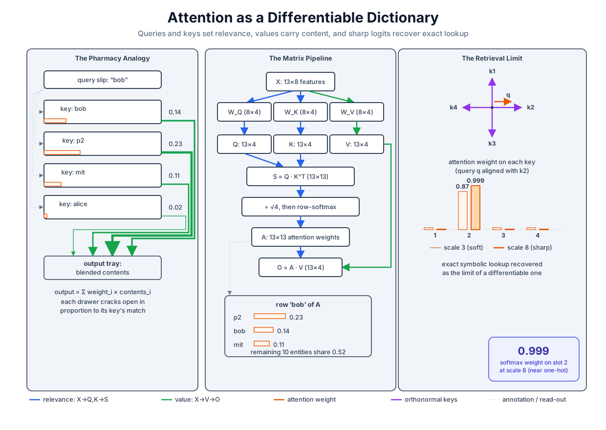Attention as a soft dictionary: queries and keys decide relevance, values carry content, the output is a relevance-weighted average, and in the orthogonal-keys sharp-logits limit the soft lookup becomes an exact one. Original diagram by the authors, created with AI assistance.

One query row, every stage: bob

Abstraction verified is abstraction earned, so here is one complete row of the pipeline, quoted verbatim from the committed run (python3 attention_demo.py). The query entity is bob, a Professor; the columns are the raw dot product $\mathbf{q}_{\text{bob}}\cdot\mathbf{k}_j$, the same after division by $\sqrt{4} = 2$, and the softmax weight:

[1] the pipeline for one query row: bob (a Professor)
  key      type         raw q·k   /√d_k   softmax
  alice    Professor     -2.3871 -1.1935    0.0248
  bob      Professor      1.0730  0.5365    0.1397
  carol    Student       -2.0115 -1.0058    0.0299
  cmu      Institution   -1.0990 -0.5495    0.0472
  dave     Student        0.1258  0.0629    0.0870
  erin     Student       -0.8574 -0.4287    0.0532
  logic    Topic         -1.4944 -0.7472    0.0387
  mit      Institution    0.5753  0.2876    0.1089
  ml       Topic         -0.4054 -0.2027    0.0667
  nesy     Topic         -3.6375 -1.8187    0.0133
  p1       Paper          0.1508  0.0754    0.0881
  p2       Paper          2.0572  1.0286    0.2286  <- top-1
  p3       Paper         -0.2016 -0.1008    0.0739
  top-3 attended: p2 (0.2286), bob (0.1397), mit (0.1089)
  output row O[bob] = A[bob]·V = [0.3032, -0.2232, 0.2016, 0.3022]
  every softmax row sums to 1: max |row_sum - 1| = 2.22e-16  (< 1e-12)

Read the trace column by column, then the summary lines. The 13 raw scores span $-3.64$ to $+2.06$; scaling halves them; the softmax turns them into a distribution that puts $0.2286$ on the paper p2, $0.1397$ on bob himself, and $0.1089$ on mit, with the remaining mass spread thinly. Bob's output row is then the corresponding mixture of the 13 value vectors, four numbers because $d_k = 4$. The final line is the sanity check that softmax rows are genuine probability distributions: over all 13 rows the largest deviation of a row sum from 1 is $2.22 \times 10^{-16}$, one unit in the last place of double precision, and the harness gates it below $10^{-12}$ (attention_demo.py line 255).

One honesty note before we lean on this row. The head is untrained: its projections are seeded $N(0, 1)$ draws, deliberately left without the usual $1/\sqrt{d}$ initialization shrink, so that even an untrained head's logits come out large enough to give a visibly non-uniform row (per the comment at attention_demo.py lines 226–229; training would normally do this sharpening). The fact that bob attends to p2 is therefore arbitrary, an accident of the seed. What is not arbitrary is the machinery: every number above follows from $X$, $W_q$, $W_k$, $W_v$ by the five lines quoted earlier, and training would move the projections so that the relevance pattern serves a task. The rest of the chapter is about the three properties of that machinery which survive any choice of weights.

Why √d_k: the variance of a dot product

The division by $\sqrt{d_k}$ looks like a fudge factor. It is a theorem about variances [3]. Model the components of a query $\mathbf{q}$ and a key $\mathbf{k}$ as independent random variables with mean zero and variance one, a reasonable stand-in for well-initialized activations, and ask how large the raw logit $z = \mathbf{q}\cdot\mathbf{k}$ typically is. Here the expectation $\mathbb{E}[\cdot]$ is the average value of a random quantity and the variance $\mathrm{Var}(\cdot) = \mathbb{E}[(\cdot)^2] - (\mathbb{E}[\cdot])^2$ is its average squared spread around that mean.

First the mean. Expectation is linear, so it passes through the sum, and independence lets the expectation of a product factor into the product of expectations:

$$\mathbb{E}[z] \;=\; \mathbb{E}\!\left[\sum_{i=1}^{d_k} q_i k_i\right] \;=\; \sum_{i=1}^{d_k} \mathbb{E}[q_i k_i] \;=\; \sum_{i=1}^{d_k} \mathbb{E}[q_i]\,\mathbb{E}[k_i] \;=\; \sum_{i=1}^{d_k} 0 \cdot 0 \;=\; 0.$$

Next the variance of one term. Using the definition of variance and then independence again:

$$\mathrm{Var}(q_i k_i) \;=\; \mathbb{E}[(q_i k_i)^2] - \big(\mathbb{E}[q_i k_i]\big)^2 \;=\; \mathbb{E}[q_i^2]\,\mathbb{E}[k_i^2] - 0 \;=\; 1 \cdot 1 \;=\; 1,$$

where $\mathbb{E}[q_i^2] = \mathrm{Var}(q_i) + (\mathbb{E}[q_i])^2 = 1 + 0 = 1$ and likewise for $k_i$. Finally, the terms $q_1 k_1, q_2 k_2, \ldots$ are built from disjoint sets of independent variables, so they are themselves independent, and the variance of a sum of independent terms is the sum of the variances:

$$\mathrm{Var}(z) \;=\; \sum_{i=1}^{d_k} \mathrm{Var}(q_i k_i) \;=\; \sum_{i=1}^{d_k} 1 \;=\; d_k.$$

So the raw logit has standard deviation $\sqrt{d_k}$: it grows with the key width, even though nothing about the task changed. Dividing by $\sqrt{d_k}$ undoes this exactly, because scaling a random variable by a constant $c$ scales its variance by $c^2$:

$$\mathrm{Var}\!\left(\frac{z}{\sqrt{d_k}}\right) \;=\; \frac{1}{d_k}\,\mathrm{Var}(z) \;=\; \frac{d_k}{d_k} \;=\; 1.$$

The demo measures the claim rather than trusting it. For each $d_k \in \lbrace 4, 64, 256\rbrace$ (the symbol $\in$ reads "is an element of" the set that follows, so $d_k$ takes each listed width in turn) it draws 10,000 independent query–key pairs with standard normal components and takes the sample variance of the dot products (attention_demo.py lines 118–123):

    for d in VAR_DIMS:
        q = rng.normal(size=(VAR_DRAWS, d))
        k = rng.normal(size=(VAR_DRAWS, d))
        dots = (q * k).sum(axis=1)
        var = float(dots.var())
        rows.append({"d_k": d, "var": var, "ratio": var / d})

The committed results sit within 3 percent of the derived value at every width:

$d_k$	sample $\mathrm{Var}(\mathbf{q}\cdot\mathbf{k})$ over 10,000 draws	ratio to $d_k$
4	3.9980	0.9995
64	63.6778	0.9950
256	262.5068	1.0254

Why does logit scale matter at all? Because the softmax is exponential in its inputs, and at $d_k = 256$ the unscaled logits have standard deviation $\sqrt{256} = 16$: among 13 keys the largest logit will typically sit tens of units above the rest, and after exponentiation one key soaks up essentially all the mass. The demo exhibits exactly this. With 13 random keys at $d_k = 256$, the committed run reports

  saturation at d_k=256 (13 keys): max softmax prob 0.9903 unscaled  vs  0.2282 with /√d_k

Unscaled, the distribution is already almost one-hot at initialization, before anything has been learned; scaled, it stays soft. The next section shows why an almost-one-hot softmax is not merely inelegant but fatal to learning: its gradient vanishes.

The softmax Jacobian, derived and checked

The softmax turns a vector of logits $\mathbf{z} = (z_1, \ldots, z_n)$ into probabilities

$$p_i \;=\; \frac{e^{z_i}}{S}, \qquad S \;=\; \sum_{k=1}^{n} e^{z_k},$$

where $e^{z}$ is the exponential function, positive for every input, which is what makes each $p_i$ positive and the row sum exactly one. (The implementation subtracts the row maximum first; writing $\mathbf{1}$ for the all-ones vector, so that $c\mathbf{1}$ shifts every logit by the same constant $c$, we have $\operatorname{softmax}(\mathbf{z}) = \operatorname{softmax}(\mathbf{z} - c\mathbf{1})$, the constant cancelling top and bottom. The shift therefore changes nothing while keeping every exponent at most zero, so the unscaled $d_k = 256$ logits above cannot overflow; attention_demo.py lines 51–61.)

To train anything through attention we need the Jacobian of this map: the matrix $J$ whose entry $J_{ij} = \partial p_i / \partial z_j$ records how output probability $i$ responds to a nudge of logit $j$. Apply the quotient rule, the derivative of a ratio $u/v$ being $(u'v - uv')/v^2$, with $u = e^{z_i}$ and $v = S$. Two ingredients: $\partial e^{z_i}/\partial z_j$ equals $e^{z_i}$ when $i = j$ and $0$ otherwise, and $\partial S/\partial z_j = e^{z_j}$ because only one term of the sum contains $z_j$.

Case $i = j$. Both the numerator and the denominator depend on $z_i$:

$$\frac{\partial p_i}{\partial z_i} \;=\; \frac{e^{z_i}\,S - e^{z_i}\,e^{z_i}}{S^2} \;=\; \frac{e^{z_i}}{S} - \left(\frac{e^{z_i}}{S}\right)^{\!2} \;=\; p_i - p_i^2 \;=\; p_i\,(1 - p_i).$$

Case $i \ne j$. The numerator $e^{z_i}$ does not depend on $z_j$, so its derivative contributes zero:

$$\frac{\partial p_i}{\partial z_j} \;=\; \frac{0 \cdot S - e^{z_i}\,e^{z_j}}{S^2} \;=\; -\,\frac{e^{z_i}}{S}\cdot\frac{e^{z_j}}{S} \;=\; -\,p_i\,p_j.$$

The Kronecker delta $\delta_{ij}$ (equal to 1 when $i = j$ and 0 otherwise) merges the two cases into one formula, and the formula assembles into one matrix:

$$\frac{\partial p_i}{\partial z_j} \;=\; p_i\,(\delta_{ij} - p_j), \qquad\text{i.e.}\qquad J \;=\; \operatorname{diag}(\mathbf{p}) - \mathbf{p}\,\mathbf{p}^\top,$$

where $\operatorname{diag}(\mathbf{p})$ is the square matrix with $\mathbf{p}$ on its diagonal and zeros elsewhere, and $\mathbf{p}\mathbf{p}^\top$ is the outer product with entries $p_i p_j$. In code this derivation is a single line (attention_demo.py lines 74–75):

    # J = diag(p) − p pᵀ   (the gradient formula derived above)
    return np.diag(p) - np.outer(p, p)

A derivation this consequential deserves an independent check, and central finite differences provide one: column $j$ of the numerical Jacobian is $\big(\operatorname{softmax}(\mathbf{z} + h\mathbf{e}_j) - \operatorname{softmax}(\mathbf{z} - h\mathbf{e}_j)\big)/(2h)$, where $\mathbf{e}_j$ is the $j$-th standard basis vector, with truncation error of order $h^2 \approx 10^{-10}$ at $h = 10^{-5}$ (attention_demo.py lines 153–158):

    h = 1e-5
    J_num = np.zeros((5, 5))
    for j in range(5):
        dz = np.zeros(5)
        dz[j] = h
        J_num[:, j] = (softmax(z + dz) - softmax(z - dz)) / (2 * h)

The committed run, on five seeded logits:

[3] softmax Jacobian  J = diag(p) - p·pᵀ  (∂p_i/∂z_j = p_i(δ_ij - p_j))
  p = softmax(z) on 5 seeded logits = [0.0204, 0.0382, 0.0611, 0.7896, 0.0907]
  J[0] = [ 0.02001, -0.00078, -0.00125, -0.01613, -0.00185]
  J[1] = [-0.00078,  0.03669, -0.00233, -0.03012, -0.00346]
  J[2] = [-0.00125, -0.00233,  0.05736, -0.04824, -0.00554]
  J[3] = [-0.01613, -0.03012, -0.04824,  0.16612, -0.07163]
  J[4] = [-0.00185, -0.00346, -0.00554, -0.07163,  0.08248]
  max |J - central finite difference| = 3.65e-12  (< 1e-6)

You can reproduce entries by hand from the printed $\mathbf{p}$. The dominant diagonal entry is $J_{33} = p_3(1 - p_3) = 0.7896 \times 0.2104 = 0.1661$, matching the printed $0.16612$ within the rounding of $\mathbf{p}$ to four decimals; the off-diagonal $J_{34} = -p_3\,p_4 = -0.7896 \times 0.0907 = -0.0716$, matching $-0.07163$ the same way. The analytic and numerical Jacobians agree to $3.65 \times 10^{-12}$, more than five orders of magnitude below the harness gate of $10^{-6}$ (attention_demo.py line 256).

Now the payoff, the connection back to the scaling. Look at what happens to $J$ as $\mathbf{p}$ approaches a one-hot vector, say $p_m \to 1$ and every other $p_i \to 0$. Every diagonal entry $p_i(1 - p_i)$ goes to zero (either factor vanishes), and every off-diagonal entry $-p_i p_j$ goes to zero too (at least one factor vanishes, since at most one index can be $m$). So $J \to 0$: the entire matrix. A saturated softmax passes no gradient whatsoever back to its logits; the relevance weights are frozen at whatever accident of initialization produced them, and no amount of training signal can move them. At the unscaled maximum probability $0.9903$ measured above, the largest possible Jacobian entry is $0.9903 \times 0.0097 \approx 0.0096$, already some twenty-six-fold smaller than the $1/4$ ceiling that $p_i(1 - p_i)$ attains at $p_i = 1/2$. The $\sqrt{d_k}$ scaling is therefore not cosmetic: it is what keeps $\mathbf{p}$ in the region where $J$ is alive and relevance remains learnable [3].

The retrieval limit: attention as exact lookup

The Jacobian argument says sharp attention cannot learn. This section shows the flip side: sharp attention can retrieve, exactly, and that limit is the bridge Part V is built to cross. Set up the cleanest possible dictionary: four slots whose keys are the rows of the identity matrix $I_4$, hence orthonormal (each of unit length, every pair at dot product zero), and four random stored values (attention_demo.py lines 177–183):

    K = np.eye(4)                        # 4 orthonormal keys (the slots)
    V = rng.normal(size=(4, 4))          # 4 stored values
    out = {}
    for c in (3.0, 8.0):
        q = c * K[2]                     # "fetch slot 2", at temperature 1/c
        p = softmax(q @ K.T)             # logits (0, 0, c, 0)
        o = p @ V

The query is $\mathbf{q} = c\,\mathbf{k}_2$: "fetch slot 2," with the scalar $c$ controlling sharpness. Orthonormality makes the logits trivial to compute by hand: $z_j = \mathbf{q}\cdot\mathbf{k}_j = c\,(\mathbf{k}_2\cdot\mathbf{k}_j) = c\,\delta_{2j}$, so the logit vector is $(0, 0, c, 0)$. The softmax then has closed form: the target slot gets $p_2 = e^{c}/(e^{c} + 3)$ and each of the other three gets $1/(e^{c} + 3)$. At $c = 3$, $e^3 = 20.09$, so $p_2 = 20.09/23.09 = 0.8700$; at $c = 8$, $e^8 = 2981$, so $p_2 = 2981/2984 = 0.9990$. The committed run confirms both, and reports the cosine similarity between the attention output and the stored value it was asked for, $\cos(\mathbf{o}, \mathbf{v}_2) = \mathbf{o}\cdot\mathbf{v}_2 / (\lVert\mathbf{o}\rVert\,\lVert\mathbf{v}_2\rVert)$, where the double bars denote the Euclidean length (the norm) of a vector, $\lVert\mathbf{u}\rVert = \sqrt{\mathbf{u}\cdot\mathbf{u}}$, so a cosine of 1 means the two vectors point the same way:

[4] dictionary-lookup limit: keys = I_4 (orthonormal), q = c·key_2
  c=3: attention = [0.0433, 0.0433, 0.8700, 0.0433]  p(slot 2)=0.8700  cos(output, value_2)=0.9807
  c=8: attention = [0.0003, 0.0003, 0.9990, 0.0003]  p(slot 2)=0.9990  cos(output, value_2)=1.0000

At $c = 3$ the lookup is genuinely soft: 13 percent of the mass leaks to the wrong slots, and the output is a blend whose cosine with the true value is only $0.9807$. At $c = 8$ each wrong slot receives three parts in ten thousand, a total leak of one part in a thousand, and the output is value 2, to cosine $1.0000$ at the printed precision (the harness gates it at $0.99$; attention_demo.py line 259). Both ingredients matter. Orthogonality ensures no wrong key receives a positive logit, so there is no crosstalk to blend in; sharpness drives the softmax to its one-hot limit, so the average degenerates to a selection. At any fixed sharpness, correlated keys leak content, and the sharpness a given accuracy demands grows without bound as the keys align (identical keys never resolve at all); orthogonality is the clean sufficient condition, giving zero crosstalk at every sharpness, while orthogonal keys at low sharpness still blur, as the $c = 3$ row shows.

Here, then, is the thesis of Part V, in one sentence: attention degenerates to exact symbolic lookup when its keys are orthogonal and its logits sharp, so a symbolic operation is recovered as the limit of a differentiable one. Everything a discrete dictionary can do, a soft dictionary can do in the limit, and unlike the discrete one it is trainable everywhere short of the limit. The tension the Jacobian exposed is real (at the exact limit the gradient is zero, so a model must approach retrieval without freezing there), but the direction of travel is now visible: a mechanism born as smooth relevance-weighting can implement lookup, and Chapter 17's soft unification will read that implementation as inference over symbols.

Multi-head attention: subspace parallelism

One head computes one relevance pattern: a single $13 \times 13$ matrix $A$ must summarize every way the entities bear on one another. But the academic world has five distinct relations (advises, authored, cites, affiliated, about), and one softmax row cannot simultaneously be "bob's advisees" and "bob's papers." The standard remedy is multi-head attention: split the model width into $h$ independent heads, run scaled dot-product attention separately in each, concatenate the outputs, and mix them with one final matrix [3]. With $d = 8$ and $h = 2$ heads of width $d_k = 4$, head $i$ gets its own projections $W_q^{(i)}, W_k^{(i)}, W_v^{(i)}$, each $8 \times 4$, and

$$O^{(i)} = \operatorname{softmax}\!\left(\frac{X W_q^{(i)} \big(X W_k^{(i)}\big)^{\!\top}}{\sqrt{d_k}}\right) X W_v^{(i)}, \qquad O_{\text{MH}} = \big[\,O^{(1)}\ \Vert\ O^{(2)}\,\big]\, W_o,$$

where $\Vert$ denotes concatenation along the feature axis and $W_o$ is an $8 \times 8$ output mix. The demo implements exactly this (attention_demo.py lines 196–204):

    heads = []
    for _ in range(2):
        Wq, Wk, Wv = (rng.normal(size=(D_MODEL, D_K)) / np.sqrt(D_MODEL)
                      for _ in range(3))
        _, _, A_h, O_h = attention(X, Wq, Wk, Wv)
        heads.append((A_h, O_h))
    concat = np.concatenate([O for _, O in heads], axis=1)   # (13, 8)
    Wo = rng.normal(size=(D_MODEL, D_MODEL)) / np.sqrt(D_MODEL)
    mh_out = concat @ Wo                                     # (13, 8)

and the committed shape trace confirms the algebra lands back where a single full-width head would:

[5] multi-head: 2 heads × d_k=4, concat, mix with W_o (8×8)
  X (13, 8) -> per head Q,K,V (13, 4) -> O_1 (13, 4), O_2 (13, 4)
  concat(O_1, O_2) (13, 8) @ W_o (8, 8) -> (13, 8)  ==  full-width single head (13, 8)
  bob's top-1 key per head: ['ml', 'logic']  (the heads attend differently)

The last line is the point. Even untrained, the two heads give bob different top-1 keys (the Topic ml in one subspace, the Topic logic in the other), because each head measures relevance with its own projection of the features: two heads, two notions of "relevant." Trained, this is the capacity that lets one head specialize into "attend to what I authored" while another becomes "attend to whom I advise": relation-specific lookup, one relation per subspace, and the seed of how a stack of heads can hold a typed graph's worth of distinct relevance patterns. Part V returns to it.

Attention is message passing on a complete graph

Part IV's message-passing template computed, for each node $i$, an aggregate of messages from its neighborhood $\mathcal{N}(i)$, a set given by the input graph, with combination weights fixed by the wiring (uniform, or degree-normalized as in a graph convolutional network, GCN). In the template below, $\mathbf{h}_i$ is node $i$'s current feature vector and $\mathbf{h}_i'$ its updated one; $\psi$ is the message function that transforms a neighbor's features into a message, $\phi$ is the update function that combines node $i$'s own state with the aggregated messages, and $w_{ij}$ is the fixed weight the wiring assigns to edge $(i, j)$. Compare that graph neural network (GNN) template with attention's output row:

$$\text{GNN:}\quad \mathbf{h}_i' = \phi\Big(\mathbf{h}_i, \sum_{j \in \mathcal{N}(i)} w_{ij}\,\psi(\mathbf{h}_j)\Big) \qquad\qquad \text{Attention:}\quad \mathbf{o}_i = \sum_{j=1}^{n} A_{ij}\,\mathbf{v}_j .$$

Structurally these are the same computation, with two substitutions. First, the neighborhood: attention sums over all $n$ nodes, so the graph is complete, every entity a neighbor of every other. Second, the weights: $w_{ij}$ was a constant of the wiring, while $A_{ij}$ is computed from the contents $\mathbf{q}_i \cdot \mathbf{k}_j$ at run time. A transformer layer is message passing on a complete graph with content-determined edge weights; graph attention networks occupy the midpoint, computing content-based weights but only over the given edges [4].

What the substitution buys is exactly what Part IV lacked: information travels between any two entities in one hop, rather than percolating through $L$ rounds of local exchange (where $L$ is the number of stacked message-passing layers), and the wiring is dynamic, a function of the learned projections rather than a constant of the input. What it costs is equally concrete. The attention matrix has $n^2$ entries, a harmless $13^2 = 169$ here but $10^{10}$ at a hundred thousand nodes, so the quadratic bill is the first thing every scalable variant renegotiates. And the mechanism has no built-in sparsity or edge types: the knowledge graph's five relations, which a relational graph convolutional network (R-GCN) honors with relation-specific message weights, have no native slot in $\operatorname{softmax}(QK^\top/\sqrt{d_k})$; a transformer must learn them into its heads or take them through its inputs. Attention buys freedom from given structure by giving up structure's guidance, and the neuro-symbolic question of Part V is how to buy some of that guidance back.

The unsolved part

Look once more at bob's output row: four numbers, $[0.3032, -0.2232, 0.2016, 0.3022]$, a convex combination of thirteen value vectors. An average is a lossy summary. From $\mathbf{o}_{\text{bob}}$ alone you cannot recover which entities contributed, in what proportion, or, and this is the sharp end, in what role. Suppose the values carried two facts worth keeping distinct: bob advises carol, and bob authored p1. Blended into one vector, the average retains a trace of carol, a trace of p1, a trace of advising and authoring, but nothing that binds carol to the advising and p1 to the authoring rather than the reverse. Attention decides relevance beautifully and then smears everything relevant into one point of $\mathbb{R}^{d}$, the set of all real vectors with $d$ coordinates; stacking heads multiplies the smears without ever pairing a filler to its role. This is the binding problem for vector representations, and within the attention formalism itself it has no answer: the mechanism owns a calculus of relevance but no calculus of structure. What would an answer even look like? An algebra on vectors with an operation that binds (role to filler, reversibly) and an operation that superposes (many bound pairs in one vector, separably), so that a single vector can hold "advises→carol, authored→p1" and give back the right filler when queried with the right role. Whether such an algebra can be made reliable at scale, inside noisy learned representations rather than clean constructions, is genuinely open; building the clean construction is the next chapter's job.

Why it matters

For the neuro-symbolic program, this chapter is the load-bearing wall. Volume 4's integrations need mechanisms that are differentiable end to end, so that logical structure can be trained by the gradient descent of Volume 1; attention is the proof that retrieval, the primitive act of looking something up in a memory, can be made differentiable without losing its exactness in the limit. The two committed numbers to carry forward are $3.65 \times 10^{-12}$ (the Jacobian is real and exact, so relevance is trainable) and cosine $1.0000$ (the limit is real and exact, so relevance can become lookup). Between them sits the design space of every transformer-based reasoner: sharp enough to retrieve the right fact, soft enough to keep learning. When Chapter 17 reads a query as a goal, keys as rule heads, and the softmax as a graded substitution, attention will have become soft unification, and the pharmacy wall of drawers will have quietly turned into a rulebook. That is the bridge from this volume's geometry to Volume 4's differentiable logic, and it is why a mechanism this small received a derivation this thorough.

Key terms

• Query / key / value: the three roles of a dictionary, relaxed to vectors: what I seek, what each slot is about, what each slot contains.
• Attention weights (matrix $A$): the row-wise softmax of scaled query–key dot products; row $i$ is a probability distribution expressing entity $i$'s relevance judgments.
• Scaled dot-product attention: $A = \operatorname{softmax}(QK^\top/\sqrt{d_k})$, $O = AV$; the output is a relevance-weighted average of values.
• √d_k scaling: division of the logits by $\sqrt{d_k}$, justified by $\mathrm{Var}(\mathbf{q}\cdot\mathbf{k}) = d_k$ for independent unit-variance components; it keeps logit variance at 1 for any key width.
• Softmax Jacobian: $J = \operatorname{diag}(\mathbf{p}) - \mathbf{p}\mathbf{p}^\top$, derived by the quotient rule; it vanishes as the softmax saturates, freezing relevance.
• Saturation: the near-one-hot regime of the softmax, reached by large-variance logits, where the maximum probability approaches 1 and gradients approach 0.
• Retrieval (dictionary-lookup) limit: with orthonormal keys and sharp logits, attention returns exactly one stored value; exact symbolic lookup as the limit of a differentiable operation.
• Multi-head attention: several attention heads run in parallel on learned subspaces, concatenated and mixed; capacity for multiple simultaneous relevance patterns, one relation per head.
• Content-addressed memory: memory read by matching contents rather than following an address or a fixed edge; the reading of attention that connects it to differentiable memory architectures.
• Binding problem: the inability of a weighted average to record which filler goes with which role; the open question this chapter hands to the next.

Where this leads

Attention gave us a differentiable where to look; it left us with no way to store what goes with what. The next chapter, Vector Symbolic Architectures, builds the missing algebra directly: high-dimensional vectors with a binding operation that pairs a role with its filler, a superposition operation that holds many bound pairs in a single vector, and an unbinding operation that gets the right filler back out, with the accuracy of the whole scheme guaranteed, and then measured, by the same kind of variance argument that gave us $\sqrt{d_k}$ here.

---

Companion code: examples/neural/attention_demo.py implements the full pipeline, the variance and saturation studies, the Jacobian check, the retrieval limit, and the multi-head shape trace, all from one seeded generator. Run python3 attention_demo.py from examples/neural/ to reproduce every number in this chapter; the acceptance harness examples/neural/validate.py re-executes its competency asserts (row sums, the 1e-6 Jacobian gate, the variance ratio, the 0.99 lookup cosine, the multi-head shapes) as part of the volume's verdict.