Weighted Model Counting: The #P Wall
📍 Where we are: Part II · Probabilistic Logic and Circuits — Chapter 5. Distribution Semantics defined a query's probability as a sum over 2,048 possible worlds, each forward-chained to its fixpoint; this chapter computes the same numbers in a different currency, as the weighted count of one small formula's models, and then meets the complexity wall that makes counting itself the hard part.
The previous chapter bought exactness at a brutal price: to answer any query, it materialized every one of the total choices of the academic world's eleven coins and ran a full forward-chaining pass inside each. That price is also strangely indifferent to the question. The query grandAdvisor(alice, carol) depends on exactly two coins, yet the enumeration flips all eleven, dragging nine irrelevant coins through 2,048 fixpoint computations. This chapter performs the standard repair, the reduction that every serious probabilistic-logic system is built on: collect the query's proofs, compile them into one propositional formula over only the coins that matter, and read the probability off that formula as a weighted model count. The reduction is exact, it turns conditioning into a ratio of two counts, and it concentrates all the difficulty into a single, precisely named problem. That is its virtue and its verdict, because the problem it concentrates everything into, counting the models of a formula, is #P-complete, harder than NP (nondeterministic polynomial time) under standard assumptions [1]. The chapter ends by measuring that wall rather than merely citing it.
Imagine an insurance office assessing the chance that a village festival gets its fireworks show. The thorough clerk from the last chapter simulates entire possible evenings: every combination of everything uncertain in the whole village, thousands of scenarios, each evening re-derived from scratch. A sharper clerk first asks what the show actually depends on and writes a single checklist: the show happens if (the barge arrives AND the permit clears) OR (the backup field is dry AND the permit clears). Only three uncertain items appear, so the clerk lists the eight ways those three items can turn out, keeps the rows where the checklist is satisfied, and adds up the kept rows' likelihoods. Same answer, far fewer rows, and a row that satisfies both halves of the checklist is still just one row, so nothing is double counted. The catch arrives with growth: every additional uncertain item on a checklist doubles the number of rows, so a checklist with twenty items already needs about a million rows, and no cleverness about how to list rows changes that arithmetic. This chapter is the sharp clerk's method, its exactness, and its bill.
What this chapter covers
- Grounding, worked end to end: the query's SLD (Selective Linear Definite-clause) resolution proofs collected by Volume 1's prover, each proof reduced to the coins it consumes, and the query formula assembled as a disjunction of conjunctions, quoted from the committed run.
- The correctness lemma, both directions: a world satisfies exactly when the query is derivable in it, argued carefully, marking where definiteness (no negation) carries the proof.
- The regrouping algebra: the world-sum reorganized by satisfying assignment, so that , the query's probability equal to its formula's weighted model count (WMC), is an identity, not an approximation; the committed table matches the 2,048-world oracle to an asserted 1e-12 and a measured 0.0.
- Weighted model counting defined and decoded: literal weights, assignment weights, the unweighted special case #SAT, and an eight-row worked trace in which the disjoint-sum problem of the previous chapter dies by construction.
- Conditioning as a ratio of two counts: , derived from conditional probability over worlds and read aloud on three committed evidence cases.
- The wall, stated with care: what the class #P is, what completeness means operationally, and why even this pipeline's negation-free DNF (disjunctive normal form) formulas sit on the hard side for exact counting.
- The wall, measured: the committed timing table on a parameterized family at coins, the enumerated assignments growing sixteenfold per step exactly as asserted, and an honest reading of toy-machine seconds.
- Where the structure hides: the compiled formulas are highly repetitive; pricing the factored evaluation by hand, about thirty operations over ten independent chain subproblems against a million enumerated assignments, exposes the gap the next chapter's circuits will exploit, without ever beating the worst case.
From 2,048 worlds to one formula
Fix the previous chapter's notation. The set of probabilistic facts (coins) is , with eleven members here; is the set of certain facts, the Horn rules, and a total choice (the symbol reads "is a subset of") is one possible world, with probability , where multiplies its terms together, picks out the coins in the chosen set (the symbol reads "is an element of" and negates it), and is coin 's stated probability. The success probability was defined as , the total weight of the worlds that derive , where the symbol pools the chosen coins, the certain facts, and the rules into one set and the turnstile means "derivable by Volume 1's forward chainer". The reduction of this chapter replaces the condition , which the oracle checks by running a reasoner inside every world, with a propositional formula that can be checked by looking at alone.
The raw material is proofs. Volume 1's SLD prover (sld.py) can enumerate every derivation of a query, not just the first, and the companion drains it (wmc.py lines 69–76):
def all_proofs(query: tuple) -> list[Proof]:
    """Every SLD derivation of ``query`` from the academic program, in the
    prover's deterministic rule/fact order.  ``sld.prove`` returns only the
    first proof; WMC needs the whole disjunction, so we drain the generator.
    Function-free and acyclic, so the enumeration terminates."""
    facts, rules = program()
    all_rules = [(fact, []) for fact in facts] + list(rules)
    return [proofs[0] for _sub, proofs in _solve([query], {}, all_rules, [0])]
Each proof is a finite tree: the query at the root, a rule application at each internal node, and facts at the leaves. For probability, only some leaves matter. A certain fact holds in every world and a built-in guard such as the colleague rule's neq test never consults the fact set at all, so neither constrains which world we are in; the leaves that do constrain it are the coins. The helper proof_coins (wmc.py lines 79–88) walks the tree and returns exactly the set of probabilistic facts one proof consumes, written .
Now introduce one Boolean variable per coin : a symbol that an assignment will set to 1 (the coin came up, ) or 0 (it did not). A single proof goes through in a world exactly when every coin it consumes is up, which is the conjunction (the large chains "and" over the whole set). The query succeeds when some proof goes through, which is the disjunction over proofs. The query formula is therefore
where the large chains "or" over all proofs of . A formula of this shape, an OR of ANDs of variables, is a DNF (disjunctive normal form), and in the probabilistic-logic literature its terms are called the query's explanations. Two edge cases fall out of the definition rather than needing patches. A proof that consumes no coins contributes the empty conjunction, which is the always-true formula ⊤, making a tautology: the query is certain, and the committed run asserts that its count equals 1 to the run's 1e-12 tolerance for the coin-free query person(erin); the value the counter computes is in fact exactly 1.0 (wmc.py lines 277–281). A query with no proofs yields the empty disjunction, the always-false ⊥, and counts to exactly 0. The compiler is five lines (wmc.py lines 114–118, inside query_dnf):
    pf = PROB_FACTS if prob_facts is None else prob_facts
    terms = {proof_coins(proof, pf) for proof in all_proofs(query)}
    dnf = _absorb(terms)
    weights = {v: pf[v] for t in dnf for v in sorted(t)}
    return dnf, weights
The _absorb step (wmc.py lines 92–99) applies the absorption law : if one term's coin set strictly contains another's, the larger term is redundant, because any assignment satisfying already satisfies , so deleting the superset term changes no assignment's verdict and therefore changes no count. Running the compiler on the four committed queries prints the actual formulas:
[1] queries compiled to weighted DNFs  φ_q = ∨_proofs ∧_coins x_f
    (a variable x_f per coin; certain facts contribute no variable)
      grandAdvisor(alice, carol)  1 proof(s) -> 1 term(s) over 2 var(s)
          φ = advises(alice, bob) ∧ advises(bob, carol)            w: 0.90, 0.90
      citesTransitively(p3, p1)   1 proof(s) -> 1 term(s) over 2 var(s)
          φ = cites(p2, p1) ∧ cites(p3, p2)                        w: 0.80, 0.90
      colleague(carol, erin)      1 proof(s) -> 1 term(s) over 1 var(s)
          φ = affiliated(erin, cmu)                                w: 0.55
      grandAdvisor(alice, Z)      2 proof(s) -> 2 term(s) over 3 var(s)
          φ = advises(alice, bob) ∧ advises(bob, carol)            w: 0.90, 0.90
            ∨ advises(alice, bob) ∧ advises(bob, dave)             w: 0.90, 0.85
Eleven coins in the program, but at most three variables in any formula. That shrinkage is the entire point, and it is what the enumeration of the previous chapter could never see.
Both directions of the lemma
Everything rests on one claim, so it deserves a real proof, not a gesture. For a total choice , write for the assignment that sets exactly when , and write (the symbol reads "satisfies") for "the assignment makes the formula true".
Lemma. For every total choice : if and only if .
One reading convention first. For a query with a variable, such as grandAdvisor(alice, Z), the turnstile means the previous chapter's existential success semantics: some ground instance of is derivable. Since all_proofs enumerates the proofs of every instance, the disjunction over proofs in already ranges over all groundings, and both directions below go through unchanged.
Derivable implies satisfies. Suppose world derives . Everything the forward chainer derives has a finite derivation tree whose leaves lie in : each atom added at round is the head of a rule whose body atoms all arrived at earlier rounds, so splice those atoms' trees together beneath that rule application, by induction on rounds (the same round-by-round induction the previous chapter used to prove monotonicity). This same tree is a valid derivation from the full program, the one with every coin available, because its leaves are facts there too: . Volume 1's SLD search, run exhaustively as all_proofs runs it, enumerates every derivation of from the full program. That word "every" is not an observation about the code but a theorem being used: by the completeness of SLD resolution for definite programs, which holds for any fixed selection rule and so for this prover's leftmost one, every derivation tree corresponds to an SLD refutation, so an exhaustive walk of the SLD search tree visits it (Volume 1's Resolution and SLD chapter builds that refutation machinery; its completeness on these programs is the backward-chaining face of the forward-chaining completeness proved in Inference and Proof). The enumeration is also finite (the program is function-free, and its one recursive rule descends the citation graph, which is acyclic), so our tree appears as some enumerated proof . Every leaf of that is a coin lies in , since the tree used only facts available in world ; hence , so sets every variable of the term to 1, that term is true, and .
Satisfies implies derivable. Suppose . Some term of the DNF is true under , which by construction means for some enumerated proof . Look at what needs in order to be a valid derivation inside world : its leaves, which are and certain facts, all available in , plus guard tests, which hold in every world because they never consult the fact set; and its internal nodes, each a rule application whose validity depends only on the rule and the children beneath it, never on which other facts exist. So the identical tree is a derivation in world , and . ∎
Mark where definiteness carried weight, because it did so twice. In the first direction, a derivation valid in the small world remained valid in the full program; that is the monotonicity the previous chapter proved for definite programs, and it is what guarantees all_proofs, which only ever sees the full program, still covers every world's proofs. In the second direction, a proof's validity depended only on its own leaves being present. Both steps break the moment negation enters: with negation as failure, a proof can depend on the absence of a fact, so a proof of the full program may fail in a smaller world and vice versa, and would need a far more careful translation with negative literals in it. This pipeline is faithful for the definite, acyclic programs the volume runs on, and claims no more.
The regrouping: from a world-sum to a model count
The lemma licenses one substitution, and then plain algebra finishes the reduction. Start from the definition and substitute the lemma's condition:
Now regroup the sum by what can actually see. Let be the set of coins whose variables occur in (three of the eleven, for grandAdvisor(alice, Z)), and split every total choice into the part the formula reads and the part it ignores: is determined by the pair , where is the restriction of to the variables of and is the set of chosen coins outside (the symbol reads "minus", set difference). Two facts make the regrouping work. First, factorizes across the split, because it is a product with one factor per coin:
Second, whether depends only on , since mentions no variable outside . So the single sum over becomes a double sum over the pairs, the satisfaction test and the factor pull out of the inner sum, and the inner sum collapses:
The remaining inner sum is over all subsets of the ignored coins, with no condition attached, and it equals a product of two-term sums: expanding the product by the distributive law generates one summand per way of picking either or for each coin, which is exactly one summand per subset , each appearing once. Therefore
and the ignored coins vanish from the answer entirely:
The right-hand side no longer mentions worlds, reasoners, or fixpoints: it is a sum over one formula's satisfying assignments of a product of per-variable weights, and it has a name.
Weighted model counting, defined
Let be a propositional formula over Boolean variables , where is the number of distinct coins the formula mentions. An assignment gives each variable a value in ; there are of them, and an assignment with is called a model of . Give every literal (a variable or its negation, written ) a weight: and . The weight of an assignment is the product of the weights of the literals it makes true, and the weighted model count, abbreviated WMC, is the total weight of the models:
The regrouping identity of the last section says precisely that with . Setting every literal weight to 1 instead recovers the unweighted special case: each model then contributes exactly 1, and the sum is the number of models, the problem called #SAT (read "sharp-SAT"). Weighted model counting is #SAT with a probability attached to each model, and this single problem has become the common currency of exact probabilistic inference: solve it well once, and a whole family of formalisms upstream is served [2].
The companion computes the definition literally (wmc.py lines 146–167, inside wmc_counted):
    variables = sorted({v for term in dnf for v in term})
    n = len(variables)
    index = {v: i for i, v in enumerate(variables)}
    # Each term as a bitmask: ω ⊨ ∧_{f∈t} x_f  ⇔  bits & mask_t == mask_t.
    masks = [sum(1 << index[v] for v in term) for term in dnf]
    # w(x_i) if bit i is 1, else 1 − w(x_i).
    p = [weights[v] for v in variables]
    q = [1.0 - weights[v] for v in variables]

    satisfied_weights: list[float] = []
    enumerated = 0
    # Integer bits = 0 .. 2^n − 1 IS the assignment ω: bit i gives ω(x_i).
    for bits in range(1 << n):
        enumerated += 1
        # P(ω) = Π_{ω(x_i)=1} p_i · Π_{ω(x_i)=0} (1 − p_i)  (independent coins)
        w = 1.0
        for i in range(n):
            w *= p[i] if bits >> i & 1 else q[i]
        # ω ⊨ φ  ⇔  some DNF term is fully true under ω.
        if any(bits & m == m for m in masks):
            satisfied_weights.append(w)
    return math.fsum(satisfied_weights), enumerated
Every integer from to is one assignment (bit gives 's value), each is weighted, each is tested against the DNF, and math.fsum keeps the final addition exactly rounded so that the 1e-12 comparisons below test semantics rather than floating-point noise. Watch the definition run on grandAdvisor(alice, Z). Its formula has three variables; abbreviate = advises(alice, bob) at , = advises(bob, carol) at , = advises(bob, dave) at , with . All eight assignments, worked by hand:
| weight of | model of ? | contributes | |||
|---|---|---|---|---|---|
| 0 | 0 | 0 | no | — | |
| 1 | 0 | 0 | no | — | |
| 0 | 1 | 0 | no | — | |
| 0 | 0 | 1 | no | — | |
| 1 | 1 | 0 | yes, term 1 | ||
| 1 | 0 | 1 | yes, term 2 | ||
| 0 | 1 | 1 | no | — | |
| 1 | 1 | 1 | yes, both terms, counted once |
The eight weights sum to (they are a probability distribution over the assignments), and the three models contribute . Compare this with the previous chapter's disjoint-sum exhibit. The naive sum of proof products, , fails because the all-true assignment satisfies both terms and gets counted twice; inclusion-exclusion repaired it by subtracting the doubly counted by hand. In the WMC formulation there is nothing to repair: the bottom row of the table is one assignment, the if any(...) line appends its weight once no matter how many terms it satisfies, and the overlap problem is dead by construction, not by correction. The committed run certifies all four queries against the 2,048-world oracle, asserting agreement within 1e-12 (wmc.py lines 290–294) and measuring, on this world, a difference of exactly zero:
      query                        vars  assign   WMC(φ_q, w)      enumeration      |diff|
      grandAdvisor(alice, carol)      2       4   0.810000000000   0.810000000000   0.0e+00
      citesTransitively(p3, p1)       2       4   0.720000000000   0.720000000000   0.0e+00
      colleague(carol, erin)          1       2   0.550000000000   0.550000000000   0.0e+00
      grandAdvisor(alice, Z)          3       8   0.886500000000   0.886500000000   0.0e+00
      overlap handled free: grandAdvisor(alice, Z)'s two terms share
      advises(alice, bob); naive Σ term-products = 1.575000000000 (>1, not a
      probability) while WMC counts each assignment once: 0.886500000000
Read the assign column against the oracle's constant 2,048: the reduction did not change the answer by a hair, and it changed the work from forward-chaining passes to at most weighted-and-tested assignments (twenty-four multiplications and eight tests, as the structure section will price it). On a toy world that saving is cosmetic. The rest of the chapter is about why, in general, it is not a rescue either.
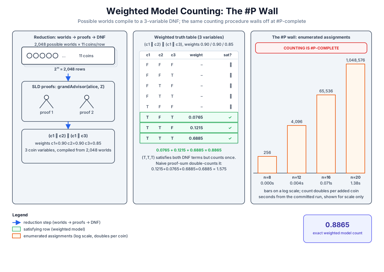 The reduction and its price: proofs compile to a three-variable DNF whose weighted models sum to the exact 0.8865, and the same counting procedure walks into an exponential wall as the variable count grows.
Original diagram by the authors, created with AI assistance.
The reduction and its price: proofs compile to a three-variable DNF whose weighted models sum to the exact 0.8865, and the same counting procedure walks into an exponential wall as the variable count grows.
Original diagram by the authors, created with AI assistance.
Conditioning is a ratio of two counts
Observing evidence is the operation that makes a probabilistic knowledge base useful, and the reduction handles it with no new machinery. The object to compute is , where the vertical bar reads "given": the probability that holds given that the evidence does. By the definition of conditional probability, for events with ,
where, over possible worlds, the joint event is "the world derives both": (abbreviating the full turnstile). Apply the lemma to each conjunct separately: derives iff , and derives iff , so derives both iff . The regrouping argument then runs word for word as before, with now the union of the two formulas' variable sets, and both numerator and denominator become counts:
One small syntactic chore remains: is a conjunction of two DNFs, not itself a DNF, so the counter cannot process it directly. The distributive law rewrites it, , one combined term per pair, followed by absorption (wmc.py lines 121–129, dnf_and). The ratio itself is then two calls to the same counter, with a third call computing the prior for display (wmc.py lines 186–193, inside conditional):
    dnf_q, w_q = query_dnf(query)
    dnf_e, w_e = query_dnf(evidence)
    w = {**w_q, **w_e}
    prior = wmc(dnf_q, w_q)
    joint = wmc(dnf_and(dnf_q, dnf_e), w)
    p_e = wmc(dnf_e, w_e)
    assert p_e > 0.0, f"evidence {evidence} has probability 0; cannot condition"
    return prior, joint, joint / p_e
This ratio-of-counts is not a trick local to logic programs; it is the same reduction by which full Bayesian-network inference was carried into weighted model counting, with each conditional-probability-table entry encoded as a weighted literal and evidence conjoined onto the query formula [3]. The committed run demonstrates it three ways on the academic world, each checked against the world-enumeration oracle to 1e-12 (wmc.py lines 313–329):
[3] conditioning = two counts: P(q | e) = WMC(φ_q ∧ φ_e, w) / WMC(φ_e, w)
      q = grandAdvisor(alice, dave)    e = grandAdvisor(alice, carol)
        P(q) = 0.765000000000   P(q ∧ e) = 0.688500000000   P(q | e) = 0.850000000000
        (e entails the proofs' shared coin advises(alice, bob), so only the
         remaining coin advises(bob, dave) = 0.85 is left standing)
      q = citesTransitively(p3, p1)    e = cites(p2, p1)
        P(q) = 0.720000000000   P(q ∧ e) = 0.720000000000   P(q | e) = 0.900000000000
        (e observes one chain link; exactly the other link cites(p3, p2) is left
         standing: posterior = 0.90)
      q = grandAdvisor(alice, carol)   e = colleague(carol, erin)
        P(q) = 0.810000000000   P(q ∧ e) = 0.445500000000   P(q | e) = 0.810000000000
        (e shares NO coin with q, so conditioning changes nothing at all
         the posterior equals the prior, to 1e-12)
Read case (a) aloud, because the numbers explain themselves once the formulas are visible. The query is "alice grand-advises dave", with in the earlier abbreviation and prior ; the evidence is "alice grand-advises carol", . Their conjunction is , with count , and the posterior is
Observing the grand-advising of carol certifies the coin the two queries share, the advising edge from alice to bob, so the only doubt left about dave is the one coin the evidence does not touch, and the posterior lands exactly on that coin's weight, up from the prior . Case (b) is idempotence doing inference: 's single conjunct, the coin cites(p2, p1), is already among 's, so the one term that distribution builds is 's own term unchanged ( at the level of coin sets), collapses back to , the joint equals the prior , and the posterior is , the other chain link. Case (c) is irrelevance made theorem-shaped: the two formulas share no variable, so by the same factorization as in the regrouping argument the joint count is the product , and the ratio hands back the prior untouched. Evidence about erin's affiliation cannot move a query about advising, and that is now an identity about variable-disjoint formulas rather than an intuition.
The wall, stated with care
Now the price. Everything above reduced inference to counting; the honest question is whether counting is easier than what we started with. The answer is a named theorem, and it needs one definition first. Many decision problems have the shape "does at least one witness exist": an instance (a formula), a polynomial-time check ("is a satisfying assignment of ?"), witnesses no longer than a polynomial in the size of . The class of such problems is NP. The class #P (read "sharp-P") contains, for each such relation, the function that maps to the number of witnesses with . Counting answers strictly more than deciding: from the count you can read off whether it is zero, so a counting oracle settles the decision problem for free, and the converse is the entire question.
| decision | counting | |
|---|---|---|
| the question about witnesses | does at least one exist? | how many exist? |
| for propositional formulas | SAT: is satisfiable? (NP-complete) | #SAT: how many models has ? (#P-complete) |
| for a monotone DNF like | trivial: make any one term's variables true | still #P-complete |
| in this chapter's pipeline | is ? one proof suffices | itself: weigh all the models |
The founding results are due to Valiant [1]: #SAT is #P-complete, meaning every counting problem in #P transforms into it in polynomial time, so an efficient exact #SAT algorithm would be an efficient exact algorithm for all of #P at once. Weighted model counting inherits the hardness immediately, since setting all literal weights to 1 turns a WMC oracle into a #SAT oracle. The third row of the table is the part that forbids wishful thinking about our particular formulas. The DNFs this pipeline compiles are monotone (no negated variable ever appears; definite programs cannot produce one), and deciding their satisfiability is trivial. Yet counting the models of a monotone DNF is already #P-complete, even when every term has only two variables [1]. Keep class and instance separate here: that result covers the chain family's class, monotone 2-DNF, but not its particular instances, whose terms deliberately share no variable and are, as the measurement section will show, easy; hard monotone 2-DNFs need terms that overlap, and the wall table below prices the enumerator's cost, not the instances' intrinsic hardness. The hardness does not live in negation or in deciding; it lives in exact counting itself, and for exact counting our friendly-looking explanation formulas sit inside the canonical hard class, not outside it. (Approximate counting is a different story on DNFs, and the closing section returns to it.)
How high does the wall reach? One honest sentence of context, stated without proof: a polynomial-time machine allowed to query a #SAT oracle can solve every problem in the entire polynomial hierarchy, the infinite tower of complexity classes stacked above NP, so the hierarchy sits inside [4]. Operationally, completeness therefore means this: a general polynomial-time weighted model counter would not be a clever data structure, it would collapse complexity theory as we currently understand it. When this volume treats exact inference as expensive, that is the theorem being deferred to.
The wall, measured
A theorem about worst cases deserves a measurement, so the companion builds a formula family where the exponential is visible and the answer is independently checkable. Take independent copies of the grandAdvisor pattern: chain connects when both of its coins come up, at and at , and the query asks whether at least one chain connects. The formula is the monotone 2-DNF over variables (wmc.py lines 220–227, inside chain_family):
    assert n % 2 == 0, "the family needs n = 2k coins"
    dnf: list[frozenset] = []
    weights: dict[tuple, float] = {}
    for i in range(n // 2):
        a, b = ("chain", str(i), "a"), ("chain", str(i), "b")
        weights[a], weights[b] = CHAIN_P
        dnf.append(frozenset({a, b}))
    return tuple(dnf), weights
Because the chains share no coin, the exact answer has a closed form to hold the counter against. One chain connects with probability and fails with probability ; the chains are independent, so all fail together with probability ; and "at least one connects" is the complement:
The committed run times the brute-force counter at :
    φ = ∨_i (a_i ∧ b_i) with w(a_i) = 0.8, w(b_i) = 0.7 — brute force
    touches ALL 2^n assignments; +4 coins = 16× the work, every time
      n    k  assignments   WMC(φ, w)        1 − 0.44^k       |diff|    seconds*
       8   4          256   0.962519040000   0.962519040000   1.1e-16     0.000
      12   6        4,096   0.992743686144   0.992743686144   1.1e-16     0.004
      16   8       65,536   0.998595177637   0.998595177637   1.1e-16     0.071
      20  10    1,048,576   0.999728026391   0.999728026391   1.1e-16     1.380
      *measured wall-clock, shown for scale only, asserted nowhere;
       the assignment COUNT (exactly 2^n, ratio 16 per step) is asserted
Read the columns honestly, because they say different kinds of things. The assignments column is machine-independent arithmetic: the counter enumerated exactly assignments, and the run asserts that each step of four coins multiplies the count by exactly (wmc.py lines 344–346). The |diff| column, at , is one unit in the last place of a double-precision float: the enumeration and the closed form agree to machine precision. The seconds column is a laptop measurement of a Python loop, shown for scale and asserted nowhere; the run-to-run numbers wobble, but the trend tracks the assignment count once past interpreter overhead (the last two steps grew by factors of about 18 and 19 against the exact 16). Extrapolate the trend, with that toy-measurement caveat attached, and remember that the inner weight loop pays multiplications per assignment: at this loop enumerates a million times as many assignments, each twice as wide, roughly two million times the cost, about a month; at , with assignments three times as wide, on the order of 150,000 years. Meanwhile the answer column creeps from toward and is, by , numerically boring. The value being computed is nearly constant; the cost of computing it by enumeration doubles per coin regardless. That mismatch, an easy-looking number priced at exponential work, is what living behind a #P wall feels like from the inside.
Where the structure hides
The brute-force column measures the algorithm, not the problem, and on these formulas the gap between the two is enormous. Look again at grandAdvisor(alice, Z): the two terms share the coin , so the distributive law factors it out,
and the factored form can be evaluated instead of enumerated. The disjunction has probability (its two variables are distinct coins, so the failure probabilities multiply), and conjoining the independent multiplies by , giving : the exact answer in five arithmetic operations, two complements, a product, a complement, a product, against the table's eight weighted rows costing twenty-four multiplications plus eight tests. The chain family is starker. Its factored evaluation needs one product per chain, one complement per chain, one running product across the complements, and a final complement: about operations, so about thirty at , against enumerated assignments each paying twenty multiplications, about twenty-one million in all. About thirty operations over ten independent chain subproblems were hiding inside a million-row enumeration, because the enumeration re-derives every chain's tiny calculation once per assignment of the eighteen coins outside it.
Both shortcuts were legitimate, and it matters exactly why. Factoring out was pure Boolean algebra; turning into a complement-of-products and into a product was sound only because, at each step, the two sides shared no variable, so their events were independent and probabilities could multiply. A compiled circuit reaches the same number by a different, more general route: it rewrites the disjunction into mutually exclusive branches, , whose events can never both fire, so plain addition of the branch counts is sound, again; that mutual exclusivity is exactly the determinism property, and the complement-of-products shortcut used above is the independence special case of that rewrite. Those two conditions, disjunction whose branches never both fire, and conjunction whose sides share no variable, are precisely the structural properties the next chapter will name (determinism and decomposability) and compile into a formula deliberately. That is the escape route: not a faster enumerator, but a one-time restructuring after which counting costs one pass over the structure. And its honest boundary is set by the theorem of the last section. Restructuring succeeds when the formula's variable interactions are local enough, when a treewidth-like width parameter of the formula stays small, and the academic world's formulas are as local as formulas get. Where the interactions are globally entangled, every known compiled form blows up exponentially (the next chapter prices exactly this succinctness trade-off across its circuit languages, and exhibits formula families whose circuits swing from linear to exponential on the choice of variable order alone), and #P-completeness is the standing reason no polynomial-time compile-and-count pipeline, present or future, can avoid the worst case unless , where is the class of functions computable in polynomial time, the function-class counterpart of the decision class P. The next chapter beats the enumeration. Nothing beats the wall.
One counting problem to rule them all
Why did an entire field agree to funnel its inference through this one hard problem? Because concentration is itself the strategy. The reduction gives every formalism upstream the same target: Bayesian networks arrive by encoding their conditional probability tables as weighted clauses, and probabilistic logic programs arrive by exactly the pipeline this chapter reenacted in miniature, the ProbLog2 pipeline: ground the program to the part relevant to the query, translate the ground program to a weighted Boolean formula, and count [5]. (Production pipelines translate to CNF, conjunctive normal form, an AND of OR-clauses that may contain negative literals; they handle cycles and negation with a more careful encoding, and they compile the formula rather than enumerating it; our DNF-of-explanations is the definite, acyclic special case with the compiler seat left deliberately empty.) The payoff of the shared target is that every improvement to counters and compilers is inherited simultaneously by logic programs, Bayesian networks, and everything else that can encode itself as a weighted formula. One problem to state, one place to optimize. And, decisive for this volume, one place to differentiate: 's sum-of-products shape is an evaluation over the algebra of real numbers, and swapping that algebra for another semiring (a number system with its own "plus" and "times" obeying the distributive law that the sum-of-products shape needs) re-answers a different question with the same structure, including, with the gradient semiring, the derivatives of the count with respect to the coin probabilities that the DeepProbLog chapter will train neural networks through.
The unsolved part
Exactness is what this chapter refused to give up, so the honest question is what surrendering it buys, and the answer depends on the shape of the formula more than on its size. For the monotone DNFs this chapter actually compiles, the news is genuinely good: exact counting stays #P-complete, but approximate counting is tractable. A classical randomized scheme estimates a DNF's count by sampling assignments term by term, and it is a fully polynomial randomized approximation scheme (FPRAS): for any accuracy and failure probability it returns, with probability at least , a value within a factor of the true count, in time polynomial in the formula size, , and , and the estimator extends to the weighted case [6]. It consults no SAT solver anywhere, because producing a model of a DNF is trivial. So the wall of this chapter forbids cheap exact answers on explanation DNFs; it does not forbid cheap guaranteed approximations of them. The hard boundary sits one encoding step away, on the CNF side where production pipelines live: approximating a CNF's model count, even quite coarsely, is NP-hard in the worst case, and the hardness persists on restricted CNF classes close to the ones reasoning produces, monotone clauses among them [7]. There, the state of the art is hashing-based counters that slice the space of models with random parity constraints and call a SAT solver as an oracle on each slice [8]; the guarantee has the same form, but it is bought with SAT calls whose worst-case time is itself exponential, so the wall is relocated into the oracle rather than removed, and the achievable time budget varies instance by instance. Approximation is a real research frontier, but it trades the unconditional guarantee for a probabilistic one, and on the CNF side it trades the fixed cost for a budget that hard instances can exhaust. This volume makes the opposite trade while it can: at academic-world scale it stays exact and asserts its numbers to 1e-12, and it says out loud that this stance does not scale. Part V of the volume will meet the other extreme, query-answering systems that never count worlds at all, and the price they pay in soundness is the volume's recurring subject.
Why it matters
Weighted model counting is where this volume's two pillars actually touch. The formula is pure symbol: it came from proofs, and its shape is the logical structure of the query's explanations. The weights are pure quantity: eleven numbers on eleven edges. is one scalar both sides agree on, and that template is what every later chapter instantiates: the circuits of the next chapter evaluate the same quantity faster, the gradient semiring differentiates it (letting a loss flow through logic into a neural network), the semantic-loss chapter penalizes a network by, in essence, the weighted count of a constraint under the network's own output probabilities, and Scallop's provenance semirings relax the same sum knowingly. The #P wall is equally load-bearing in the other direction: it is the theorem-backed reason the field's menu splits into exact-but-small and scalable-but-unsound, rather than that split being an engineering accident someone will fix next year. When Volume 5 audits trust and calibration, the systems that can show an exact count will be the ones with receipts, and the systems that scale will be the ones that must be probed empirically because they cannot. This chapter is where that fork is priced.
Key terms
- Grounding: replacing derivability-in-a-world by a propositional formula over the query's relevant coins; here, collecting all SLD proofs and keeping each proof's coin set.
- Query formula / DNF of explanations (): the disjunction, over proofs, of the conjunction of each proof's coins; a world satisfies it exactly when the query is derivable there.
- Absorption: the law ; deleting superset terms changes no assignment's verdict and no count.
- Model / satisfying assignment: an assignment of 0/1 to every variable that makes the formula true.
- Weighted model counting (WMC): ; with it equals the success probability, .
- #SAT: the unweighted special case, counting a formula's models; the counting analogue of SAT.
- #P and #P-completeness: the class of witness-counting functions for NP relations; #SAT is complete for it, monotone 2-DNF counting included, and the polynomial hierarchy sits inside , so efficient exact counting would collapse it.
- FPRAS (fully polynomial randomized approximation scheme): an algorithm returning, with probability at least , an answer within a factor of the truth, in time polynomial in the input size, , and ; DNF counting has one, CNF counting has none unless standard assumptions fail.
- Conditioning as two counts: , with the conjunction rebuilt as a DNF by distribution plus absorption.
- The chain family: independent two-coin chains, ; closed form , brute-force cost exactly assignments.
Where this leads
The chapter ends on a deliberate imbalance: the same formula that brute force pays a million assignments for was evaluated by hand in about thirty operations, because its disjunctions never double-counted and its conjunctions never shared variables. The next chapter, Circuits: SDD, d-DNNF, and Fast Evaluation, turns that observation into an engineering discipline called knowledge compilation: pay once to restructure the formula into a circuit whose OR-nodes are deterministic and whose AND-nodes are decomposable, then answer by a single bottom-up pass, linear in the circuit's size. On this chapter's certified formulas, the committed compiler reproduces every count to machine precision and dispatches the chain family in 238 circuit operations instead of 1,048,576 assignments. It beats the enumeration soundly. The worst case it leaves standing, exactly where this chapter proved it must.
Companion code: examples/integration/wmc.py compiles queries to weighted DNFs with Volume 1's sld.py prover, counts by literal enumeration, conditions by two counts, certifies every academic-world number against distsem.py's 2,048-world oracle within 1e-12, and certifies the wall table's values against the closed form within 1e-9; its asserts also pin the overlap exhibit, all three conditioning cases, and the exact assignment counts of the wall table (timings alone are never asserted). Run python3 examples/integration/wmc.py to reproduce every asserted number quoted above (the seconds column varies by machine).