Semantic Loss and Constraint Layers

📍 Where we are: Part III · Differentiable Frameworks — Chapter 8. DeepProbLog put a neural network under a logic program and trained it through exact inference; this chapter aims the same circuit machinery at plain supervised learning, where the logic is not a program above the network but a constraint on the network's own outputs.

Part II built a pipeline for computing the probability of a logical query: possible worlds, weighted model counting, compiled circuits, and a gradient that rides along in the same pass. Every use so far has pointed that pipeline at a knowledge base. This chapter points it at something much more ordinary: a classifier. You are training a network with several output units, and you know something about the output space that no individual label says. Exactly one of the class bits should be on. A paper flagged neuro-symbolic must also be flagged logic. That knowledge is a propositional formula over the output variables, and the question is where, in a gradient-trained model, such a formula can enter. The answer developed here is the semantic loss: the constraint becomes a differentiable penalty equal to the negative logarithm of the probability that the network's own outputs, read as independent coin flips, land on a state satisfying the constraint. The definition is short, provably the only one satisfying three natural axioms, and computable by exactly the weighted-model-counting machinery already on the table. At the end we flip the axis: a loss makes violations expensive, a constraint layer makes them impossible, and both price the same quantity.

The simple version

Imagine a student filling in a multiple-choice bubble sheet, one correct bubble per row. A tutor grading over their shoulder has the answer key for only a few rows. But the tutor can still say something useful about every row: a row with two bubbles filled is wrong no matter what the key says, and so is a row left blank. So the tutor charges two kinds of penalty: "that answer contradicts the key" on the few keyed rows, and "that answer contradicts the format" on all of them. Over time the format penalty alone makes the student decisive and consistent, and the few keyed rows anchor which decisive answers are right. The semantic loss is the format penalty, made differentiable. The constraint layer at the end of the chapter is a stricter tutor: it redesigns the sheet so that filling two bubbles in one row is physically impossible.

What this chapter covers

• The design question: you know a constraint α over the output space; three doors let it into a gradient-trained model (a fuzzy penalty, a probabilistic loss, a hard layer), and the naive fourth door, penalizing violations of the argmax, is closed by the mathematics of differentiation itself.
• The definition, decoded then formal: the semantic loss $L^s(\alpha, p) = -\log \mathrm{WMC}(\alpha; p)$, where WMC is the weighted model count of Part II: the self-information of sampling a satisfying state from the network's per-variable sigmoids, and why the source's sigmoid-not-softmax output layer is load-bearing.
• Three axioms, one loss: monotonicity under entailment, zero cost for a state against itself, and proportionality to cross-entropy on single literals pin the definition down uniquely up to a constant (given the regularity conditions the source adds), with syntax independence arriving not as another axiom but as a derived guarantee; the conditions themselves are checked as committed code.
• Exactly-one, worked in full: the weighted model count collapses to the closed form $\sum_i p_i \prod_{j \ne i} (1 - p_j)$, the gradient is derived term by term, traced numerically at a concrete point, and certified against central finite differences at 3.6e-11.
• The general recipe: an arbitrary constraint compiles once into the circuit of Circuits; the forward pass is WMC, and the gradient needs no separate backward pass: it rides the same single pass with the circuit evaluated under the gradient semiring instead, loss and gradient linear in circuit size per batch (the pair evaluation carries a gradient vector per node, a factor of the number of output bits).
• The committed experiment: 12 labeled points, 180 unlabeled points, and one exactly-one constraint; cross-entropy alone versus cross-entropy plus the semantic loss, compared on accuracy and on constraint-violation rate.
• Losses versus layers: the design fork between penalizing violations during training and renormalizing them away at test time, with the Semantic Probabilistic Layer and the hierarchy layer as the constructive alternatives, and one table pricing the trade.

Three doors, and the one that will not open

Fix the setting precisely. A network ends in $k$ output units, where $k$ is the number of labels; here $k = 3$, and the three labels are the academic world's topics logic, ml, nesy, imported from Volume 3's kg.py and never retyped (semantic_loss.py lines 87–89). Attach to each unit a Boolean output variable $X_i$, a variable taking only the values true and false, read as "the network asserts label $i$." A constraint $\alpha$ is a propositional formula over $X_1, \ldots, X_k$: exactly one topic is on, or a paper flagged nesy is also flagged logic. The design question is where $\alpha$ can enter the training of the network's parameters $\theta$ (the weights and biases gradient descent updates).

The tempting first answer is to bolt a penalty onto the discrete prediction: decode the outputs to hard labels by an argmax (the index of the largest output) or by thresholding each unit at $\tfrac12$, and add a fine whenever the decoded labels violate $\alpha$. Count the ways this fails. First, the map from continuous outputs to the argmax is piecewise constant: nudge the outputs a little and the winning index does not change, so the penalty's derivative with respect to the outputs is zero at almost every point. Second, at the boundary points where the argmax does change, the penalty jumps discontinuously, so no derivative exists there at all. Third, the violation test itself is a zero-one indicator, another step function stacked on the first. The chain rule multiplies these stages, and a product with a zero factor is zero: whatever $\theta$ does, the gradient of the penalty is $0$ wherever it is defined. Gradient descent, which sees the world only through gradients, is structurally blind to such a penalty. Any usable design must couple $\alpha$ to the continuous outputs, before any decoding.

Three doors do exactly that, and this volume walks through all of them. The fuzzy door is Part I's: read each output $p_i$ as a degree of truth, replace AND ($\wedge$), OR ($\vee$), and NOT (¬) by the t-norm operators, evaluate $\alpha$ to a number in $[0,1]$, and penalize its shortfall from $1$. It is differentiable, but the penalty depends on which t-norm you chose and on how the formula happens to be written. The probabilistic door is this chapter's: read the outputs as probabilities of independent Boolean variables and charge the network the negative logarithm of the probability that $\alpha$ holds [1]. The structural door is the closer's: change the model rather than the loss, ending the network in a layer that can only emit distributions over $\alpha$'s satisfying states, so violations are not discouraged but impossible [2].

The definition: the surprise of sampling a satisfying state

Decode the probabilistic reading before the formula. The network's output layer applies a sigmoid $\sigma(z) = 1/(1 + e^{-z})$ to each of the $k$ logits (the raw pre-sigmoid output numbers, one per label) independently, producing $\mathbf{p} = (p_1, \ldots, p_k)$ with each $p_i \in [0,1]$; here $e^{-z}$ is the exponential function, Euler's number $e \approx 2.718$ raised to the negated logit $-z$, so a large positive logit drives $e^{-z}$ toward zero and $\sigma(z)$ toward $1$. Treat each $p_i$ as the parameter of an independent coin: flip all $k$ coins, and the result is a state $\mathbf{x} \in \lbrace 0,1 \rbrace^k$, an assignment of true (1) or false (0) to every output variable. Under independence, the probability of a particular state is the product of its per-coordinate probabilities,

$$P_{\mathbf{p}}(\mathbf{x}) \;=\; \prod_{i=1}^{k} p_i^{x_i}\,(1 - p_i)^{1 - x_i},$$

where the exponent trick just selects the right factor: coordinate $i$ contributes $p_i$ when $x_i = 1$ and $1 - p_i$ when $x_i = 0$. Write $\mathbf{x} \models \alpha$ (the symbol $\models$ reads "satisfies") for the states on which the formula $\alpha$ is true; these are $\alpha$'s models. The semantic loss is the negative logarithm of the total probability that the sampled state is a model [1]:

$$L^s(\alpha, \mathbf{p}) \;=\; -\log \sum_{\mathbf{x} \models \alpha} \; \prod_{i:\, \mathbf{x} \models X_i} p_i \prod_{i:\, \mathbf{x} \models \neg X_i} (1 - p_i).$$

Now look at the sum with Part II's eyes. A sum over the models of a formula, of products of per-variable weights, with weight $p_i$ on the literal $X_i$ and weight $1 - p_i$ on the literal $\neg X_i$, is verbatim the weighted model count of Weighted Model Counting. Nothing about the definition is new machinery:

$$L^s(\alpha, \mathbf{p}) \;=\; -\log \mathrm{WMC}(\alpha;\, \mathbf{p}), \qquad w(X_i) = p_i,\;\; w(\neg X_i) = 1 - p_i.$$

The information-theoretic reading gives the loss its character: $-\log$ of a probability is the self-information of the event, the surprise (measured in nats, the natural-logarithm unit) of observing it. The semantic loss is the network's surprise that its own outputs, sampled coordinate-wise, satisfy the constraint. A network already certain of a satisfying state feels no surprise and pays nothing; a network whose outputs make satisfaction improbable pays heavily; a network whose outputs make satisfaction impossible would pay infinitely, which is why the implementation clamps the count at $10^{-12}$ before the logarithm (semantic_loss.py line 107 and lines 161–165):

def semantic_loss(P: np.ndarray) -> np.ndarray:
    """L^s(α₁, p) = −log WMC(α₁; p), batched; the log is clamped at CLAMP so
    a crisply violating p (WMC = 0) prints a large finite loss instead of raising —
    a numerical-stability guard the paper's released code omits (it takes tf.log of the raw count)."""
    return -np.log(np.maximum(exactly_one_wmc(P), CLAMP))

One implementation choice is load-bearing and worth stating out loud: the output layer is $k$ sigmoids, not a softmax, exactly as in the source system's semi-supervised code [1] (the companion's docstring records this at semantic_loss.py lines 17–19). A softmax already is a single categorical distribution: sampling from it yields one class, which corresponds to a one-hot state, which satisfies exactly-one automatically. Under a softmax reading, the mass on satisfying states is $1$, the loss is identically $0$, and the constraint has no gradient to give. Independent sigmoids are what make the constraint contentful: the coins can land on zero classes, or two, and the loss exists precisely to charge for that possibility. The sigmoid reading also generalizes: multi-label settings, where several bits may legitimately be on and the constraint is an implication between labels, need no change at all.

The committed run opens by evaluating the loss on four hand-readable output vectors for the exactly-one constraint $\alpha_1$ over the three topic bits:

[1] exactly-one in closed form: WMC(α₁; p) = Σ_i p_i Π_{j≠i}(1 − p_j)
      p = (logic, ml, nesy)       WMC(α₁;p)   L^s = −log WMC
      one-hot (1.0, 0.0, 0.0)       1.000000       0.000000  Axiom 2: satisfying state, zero loss
      uniform (0.5, 0.5, 0.5)       0.375000       0.980829
      two-hot (1.0, 1.0, 0.0)       0.000000      27.631021  crisp violation: loss = −log(clamp)
      mixed   (0.2, 0.5, 0.9)       0.410000       0.891598

Each row is checkable by hand, and the next-but-one section derives the closed form that computed the middle column. The one-hot row puts all its mass on a model, so the count is $1$ and the loss $-\log 1 = 0$. The uniform row spreads mass evenly over all $2^3 = 8$ states, of which three are models, each of mass $(\tfrac12)^3$: the count is $\tfrac38 = 0.375$. The two-hot row is a crisp violation: no model receives any mass, the count is exactly $0$, and the clamp converts the infinite penalty into $-\log 10^{-12} = 12 \ln 10 = 27.631021$. The mixed row is where training actually lives, and we return to it twice.

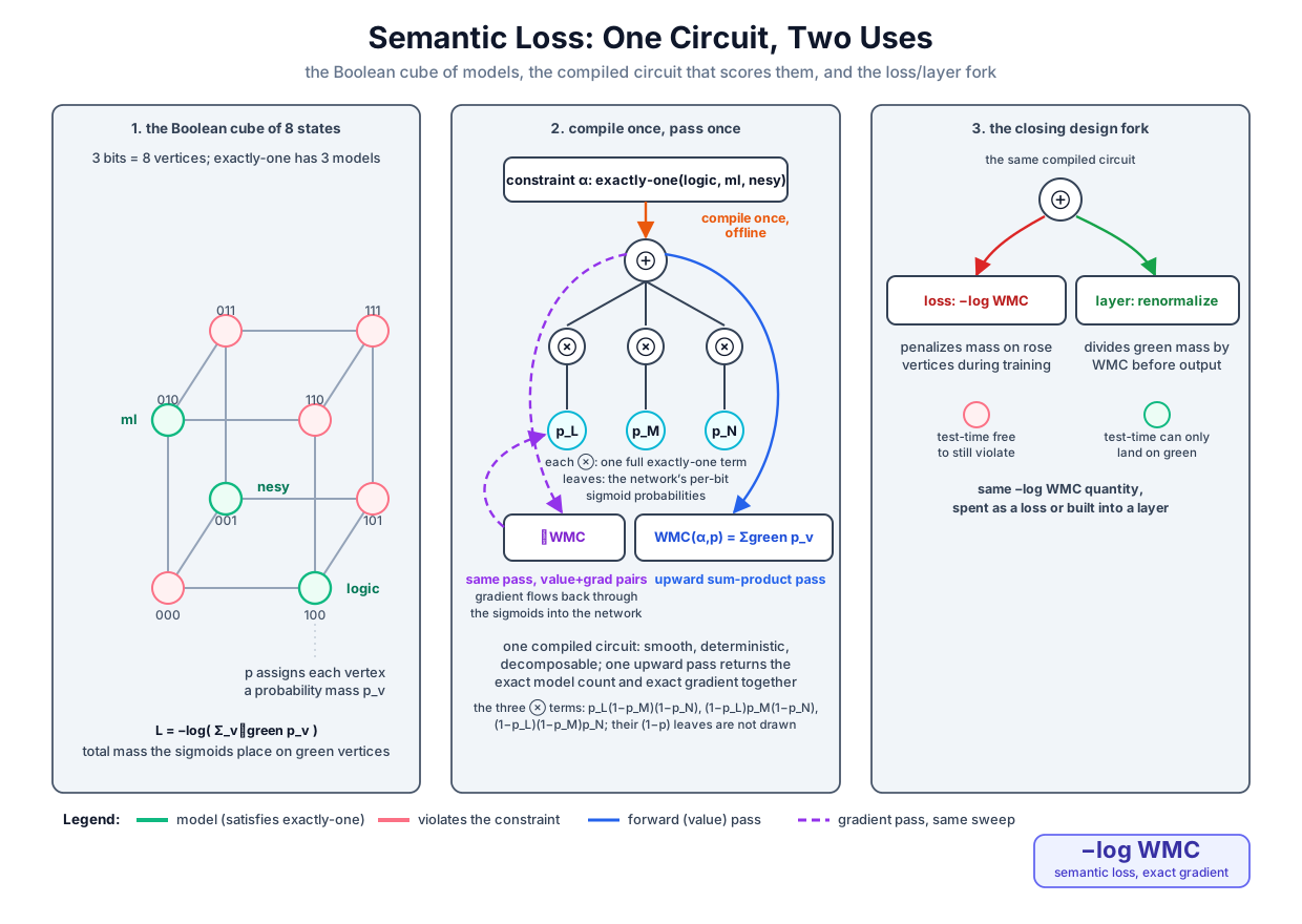The semantic loss charges the network −log of the probability mass its own sigmoids place on the constraint's models; one compiled circuit computes that mass and its gradient in a single pass, and the closing fork chooses between penalizing the violating mass (a loss) and renormalizing it away (a layer).

Original diagram by the authors, created with AI assistance.

Three axioms, one loss

Why this penalty and not another? Many differentiable functions vanish on satisfying states and grow on violating ones; the fuzzy door alone offers a whole menu. The semantic loss's answer is an axiomatic one: state what any reasonable constraint loss must do, and prove that the axioms leave no choice [1]. The source's main text states three substantive axioms plus a differentiability axiom, and its appendix adds further regularity axioms (additivity across independent sentences, among others) for the uniqueness theorem; syntax independence is then derived, not assumed. Here are the three substantive axioms and the derived guarantee, each in plain language first, with the derived one marked.

condition	plain statement	what it pins down
Axiom 1: monotonicity	a stricter constraint can never cost less: if $\alpha \models \beta$ (every state satisfying $\alpha$ satisfies $\beta$), then $L(\alpha, \mathbf{p}) \ge L(\beta, \mathbf{p})$	the loss must order constraints by their model sets, ruling out penalties that reward adding clauses
Axiom 2: identity	a state costs nothing against itself: $L(\mathbf{x}, \mathbf{x}) = 0$ for every state $\mathbf{x}$, read as its own one-model constraint	anchors the zero: no phantom penalty on success (with Axiom 1 and the appendix's Truth axiom this extends to zero loss on every satisfying state, the form the companion asserts)
Axiom 3: cross-entropy on literals	on the simplest constraint, a single literal $X_i$, the loss is proportional to the ordinary cross-entropy $-\log p_i$	fixes the functional form: the logarithm enters here, and with it the constant $c$
Derived: syntax independence	logically equivalent formulas get identical loss: $L$ depends only on which states satisfy $\alpha$, never on how $\alpha$ is spelled	the source's Proposition 2, not a separate axiom: monotonicity run in both directions of a mutual entailment forces equal loss, which is what rules out every t-norm evaluation, whose value changes with the spelling

The theorem is that these three axioms (together with the source's differentiability axiom and the further regularity conditions of its appendix, such as additivity across independent sentences and the Truth axiom, zero loss on the tautology) admit exactly one family: every loss satisfying them is $c \cdot L^s$ for a positive constant $c$ [1]. We do not reproduce the proof; it lives in the source's appendix, and the honest content for us is the axioms and what each one removes. Start with what monotonicity alone already forces. If $\alpha$ and $\beta$ are logically equivalent, each entails the other; applying the axiom in both directions gives $L(\alpha, \mathbf{p}) \ge L(\beta, \mathbf{p})$ and $L(\beta, \mathbf{p}) \ge L(\alpha, \mathbf{p})$, and two opposite inequalities force equality. That is Proposition 2, syntax independence: the loss is a function of the pair (model set of $\alpha$, $\mathbf{p}$) only, so it can only consume the masses of states, never the shape of the formula. Identity anchors the zero, and combining it with monotonicity yields the derived satisfaction property: if a state $\mathbf{x}$ satisfies $\alpha$, the conjunction of literals naming $\mathbf{x}$ entails $\alpha$, so monotonicity gives $L(\alpha, \mathbf{x}) \le L(\mathbf{x}, \mathbf{x})$, which Axiom 2 makes zero. One more premise, non-negativity, closes the argument, and it is derived rather than assumed outright: the appendix's Truth axiom sets $L(\text{true}, \mathbf{p}) = 0$ (the tautology, satisfied by every state, costs nothing), and every formula $\alpha$ entails true, so monotonicity gives $L(\alpha, \mathbf{p}) \ge L(\text{true}, \mathbf{p}) = 0$ at every $\mathbf{p}$; this is the source's Proposition 7. Combined with the bound $L(\alpha, \mathbf{x}) \le 0$ just derived, the two inequalities force $L(\alpha, \mathbf{x}) = 0$. The literal axiom then fixes the function on the one-variable family: for $\alpha = X_i$ the satisfying states are all $\mathbf{x}$ with $x_i = 1$, and their total mass factorizes. Group the $2^{k-1}$ satisfying states by their remaining free bits; the distributive law turns the sum of products into a product of sums, with one factor $p_j + (1 - p_j) = 1$ for each other coordinate:

$$\sum_{\mathbf{x}:\, x_i = 1} P_{\mathbf{p}}(\mathbf{x}) \;=\; p_i \prod_{j \ne i} \big(p_j + (1 - p_j)\big) \;=\; p_i,$$

so demanding proportionality to the cross-entropy $-\log p_i$ on literals is precisely demanding proportionality to $-\log(\text{satisfying mass})$ there. Monotonicity extends the form coherently to all formulas: a stricter constraint has a subset of the models, hence at most the mass, hence at least the $-\log$, which is exactly how the axiom says a loss must behave.

The companion refuses to leave the axioms as prose: two of the three, plus the derived guarantee, run as code. Identity, in its derived satisfying-state form, is the one-hot row of the table above, asserted at semantic_loss.py lines 446–448. Syntax independence is checked as Proposition 2, by compiling $\alpha_1$ into a circuit (a different syntax for the same meaning) and demanding the closed form back, value and gradient, to $10^{-12}$; the committed run reports agreement at $2.22 \times 10^{-16}$ (lines 461–469). Monotonicity is checked by building the conjunction $\alpha_3 = \alpha_1 \wedge \alpha_2$ (exactly one topic, and the nesy-implies-logic hierarchy of the next-but-one section), which entails both conjuncts, and asserting $L^s(\alpha_3, \mathbf{p}) \ge \max(L^s(\alpha_1, \mathbf{p}), L^s(\alpha_2, \mathbf{p}))$ at five random $\mathbf{p}$ (lines 488–495):

      Axiom 1 (monotonicity), α₃ ⊨ α₁ and α₃ ⊨ α₂, at 5 random p:
        e.g. p = (0.285, 0.319, 0.783):  L^s(α₃) = 2.3893  ≥  L^s(α₁) = 0.7491,  L^s(α₂) = 0.8195

Exactly-one, collapsed and differentiated

For the workhorse constraint the general sum needs no compiler, because the models can be listed. The exactly-one constraint $\alpha_1$ over $k$ bits is satisfied by precisely the $k$ one-hot states $\mathbf{e}_i$, where $\mathbf{e}_i$ is the state with bit $i$ on and every other bit off. Evaluate the product formula on the model $\mathbf{e}_i$: coordinate $i$ is true and contributes $p_i$; every coordinate $j \ne i$ is false and contributes $1 - p_j$. Summing the $k$ model masses, the weighted model count collapses to a closed form with $k$ terms instead of $2^k$:

$$\mathrm{WMC}(\alpha_1;\, \mathbf{p}) \;=\; \sum_{i=1}^{k} p_i \prod_{j \ne i} (1 - p_j).$$

This is what exactly_one_wmc computes, building each product $\prod_{j \ne i}(1 - p_j)$ by excluding column $i$ rather than dividing, so that a $p_j = 1$ cannot produce a zero-by-zero division (semantic_loss.py lines 118–128). The table's rows follow: at the uniform point each term is $\tfrac12 \cdot \tfrac12 \cdot \tfrac12$, three terms give $0.375$; at the mixed point $\mathbf{p} = (0.2, 0.5, 0.9)$,

$$\mathrm{WMC} \;=\; 0.2 \cdot 0.5 \cdot 0.1 \;+\; 0.5 \cdot 0.8 \cdot 0.1 \;+\; 0.9 \cdot 0.8 \cdot 0.5 \;=\; 0.01 + 0.04 + 0.36 \;=\; 0.41,$$

matching the printed $0.410000$ and $L^s = -\ln 0.41 = 0.891598$.

Now the gradient, by hand, term by term. Abbreviate $q_j = 1 - p_j$ (the off-probability of bit $j$), and fix the coordinate $m$ we differentiate with respect to. Split the sum by whether a term owns index $m$. The $i = m$ term is $p_m \prod_{j \ne m} q_j$: it is linear in $p_m$, with coefficient $\prod_{j \ne m} q_j$, so its derivative is that coefficient. Every other term, $i \ne m$, contains $p_m$ only through the single factor $q_m$: writing it as $p_i \, q_m \prod_{j \ne i,\, j \ne m} q_j$ and using $\frac{d q_m}{d p_m} = -1$, its derivative is $-\,p_i \prod_{j \ne i,\, j \ne m} q_j$. Adding the one positive piece and the $k - 1$ negative pieces:

$$\frac{\partial\, \mathrm{WMC}}{\partial p_m} \;=\; \prod_{j \ne m} q_j \;-\; \sum_{i \ne m} p_i \prod_{j \ne i,\, j \ne m} q_j.$$

The loss adds one more link. For $L^s = -\log u$ with $u = \mathrm{WMC}$, the outer derivative is $\frac{d}{du}(-\log u) = -\tfrac1u$, so the chain rule gives

$$\frac{\partial L^s}{\partial p_m} \;=\; -\,\frac{1}{\mathrm{WMC}(\alpha_1; \mathbf{p})}\, \frac{\partial\, \mathrm{WMC}}{\partial p_m}.$$

Both formulas are transcribed, with this derivation sitting in the docstring, at semantic_loss.py lines 131–158 (exactly_one_wmc_grad) and 168–174 (semantic_loss_grad). Trace them at the mixed point, where $\mathbf{q} = (0.8, 0.5, 0.1)$, working every product:

$$\frac{\partial\, \mathrm{WMC}}{\partial p_{\text{logic}}} = 0.5 \cdot 0.1 - (0.5 \cdot 0.1 + 0.9 \cdot 0.5) = 0.05 - 0.50 = -0.45,$$ $$\frac{\partial\, \mathrm{WMC}}{\partial p_{\text{ml}}} = 0.8 \cdot 0.1 - (0.2 \cdot 0.1 + 0.9 \cdot 0.8) = 0.08 - 0.74 = -0.66,$$ $$\frac{\partial\, \mathrm{WMC}}{\partial p_{\text{nesy}}} = 0.8 \cdot 0.5 - (0.2 \cdot 0.5 + 0.5 \cdot 0.8) = 0.40 - 0.50 = -0.10,$$

and dividing by $-\mathrm{WMC} = -0.41$ gives $\partial L^s / \partial \mathbf{p} = (1.0976,\, 1.6098,\, 0.2439)$. Read the direction before moving on, because it corrects a tempting intuition. All three partials are positive, so a descent step $\mathbf{p} \leftarrow \mathbf{p} - \eta\, \nabla L^s$, where $\eta$ is the step size (the learning rate) and the gradient $\nabla L^s$ is the vector of the three partial derivatives just computed, lowers all three probabilities, the ambiguous $p_{\text{ml}} = 0.5$ fastest, and even the confident $p_{\text{nesy}} = 0.9$ slightly. The gradient is not "move toward the nearest one-hot, coordinate by coordinate"; it is "increase the satisfying mass," and at this point raising $p_{\text{nesy}}$ further would cost mass, because it multiplies the $q_{\text{nesy}} = 0.1$ factor inside the logic and ml models down toward zero faster than it grows the nesy model. Once the competing bits have been muted (say $\mathbf{p} = (0.1, 0.1, 0.9)$, where the same formula gives $\partial\,\mathrm{WMC}/\partial p_{\text{nesy}} = 0.81 - 0.18 = +0.63$), the sign flips and descent drives $p_{\text{nesy}}$ up to $1$: first silence the rivals, then commit. The loss choreographs a soft argmax without ever computing one.

Hand derivations earn trust by surviving an independent oracle. The companion certifies every analytic gradient in this chapter against central finite differences, the symmetric form of the derivative's definition: for each coordinate, $\big(f(\mathbf{p} + h\mathbf{e}_m) - f(\mathbf{p} - h\mathbf{e}_m)\big) / 2h$ with $h = 10^{-5}$, accurate to order $h^2$ (semantic_loss.py lines 177–187), with every check required to agree within $10^{-6}$ (line 105). The committed run reports:

[2] gradient certificates: analytic vs central differences (h = 1e-5)
      exactly-one  ∂L^s/∂p, 5 random p              max|Δ| = 3.59e-11   PASS (≤ 1e-6)
      implication  ∂L^s/∂p via the circuit, 6 p     max|Δ| = 1.12e-09   PASS (≤ 1e-6)
      MLP backprop ∂(CE + w·L^s)/∂θ, 12 coords      max|Δ| = 6.34e-11   PASS (≤ 1e-6)

The first line is the derivation above, agreeing with the numeric oracle to $3.59 \times 10^{-11}$ at five random interior points. The second and third lines belong to the next two sections.

The general recipe: compile once, count and differentiate in one pass

Exactly-one was kind: its models could be listed. A general $\alpha$ is not kind. The sum defining $\mathrm{WMC}$ ranges over up to $2^k$ states, and Weighted Model Counting established that computing it on a raw formula is #P-complete (the counting complexity class of Part II's wall: as hard as counting the satisfying assignments of a Boolean formula). The escape is the one Circuits built: compile $\alpha$ once, offline, into a smooth deterministic decomposable circuit, and thereafter every evaluation is a single bottom-up pass, one semiring operation per edge. The source system compiles its constraints into Sentential Decision Diagrams (SDDs), shipped precompiled and evaluated through the PyPSDD library [1]; the companion stands in with circuit.compile (circuit.py lines 322–332), the Shannon-expansion compiler whose structural certificates (decomposability, determinism, smoothness) the circuits chapter checked as code, and which semantic_loss.py re-checks on every constraint it compiles (lines 418–427).

The forward pass is the count: evaluate the circuit under the probability semiring $(+, \times)$ with leaf weights $(p_i,\, 1 - p_i)$, and the root value is $\mathrm{WMC}(\alpha; \mathbf{p})$, at a cost of exactly one operation per circuit edge (circuit.py lines 336–366; the harness asserts ops == edges). The gradient needs no separate backward pass: evaluate the same circuit under the gradient semiring over pairs $(v, \nabla v)$ instead, the device DeepProbLog used to differentiate exact inference, whose pair payload makes the derivative ride along with the value. Its two operations are the sum rule and the product rule of calculus, frozen into an algebra:

$$(a, \nabla a) \oplus (b, \nabla b) = (a + b,\; \nabla a + \nabla b), \qquad (a, \nabla a) \otimes (b, \nabla b) = (a b,\; a\,\nabla b + b\,\nabla a),$$

with leaves labeled $X_c \mapsto (p_c,\, \mathbf{e}_c)$ and $\neg X_c \mapsto (1 - p_c,\, -\mathbf{e}_c)$, where $\mathbf{e}_c$ is the standard basis vector with a $1$ in coordinate $c$ and zeros elsewhere, encoding $\partial p_c / \partial p_c = 1$ and $\partial (1 - p_c) / \partial p_c = -1$ (semantic_loss.py lines 206–234). One pass then returns the count and its full gradient together, and the chain rule through the logarithm finishes the loss (semantic_loss.py lines 237–247):

def circuit_sl(circ, p: np.ndarray) -> tuple[float, float, np.ndarray]:
    """The general semantic-loss recipe on a compiled circuit: ONE
    gradient-semiring pass gives WMC(α; p) and ∇_p WMC, then the chain rule
    through the −log (as in ``semantic_loss_grad``) gives the loss gradient:

        L^s = −log WMC,   ∂L^s/∂p = −(∇_p WMC) / WMC .

    Returns (L^s, WMC, ∂L^s/∂p)."""
    wmc, g = evaluate(circ, grad_weights(p), GRAD)
    wmc = max(wmc, CLAMP)
    return -math.log(wmc), wmc, -g / wmc

The demonstration constraint is the running example's own label hierarchy: $\alpha_2 = X_{\text{nesy}} \rightarrow X_{\text{logic}}$, "a paper flagged neuro-symbolic must also be flagged logic," written as the disjunction $\neg X_{\text{nesy}} \vee X_{\text{logic}}$ (semantic_loss.py line 203). Its count also has a hand oracle, worth deriving because implications recur everywhere. Exactly one pattern of bits violates an implication: antecedent true, consequent false. Over three bits the violating states are the two with $x_{\text{nesy}} = 1$ and $x_{\text{logic}} = 0$, with $x_{\text{ml}}$ free, and their combined mass factorizes over the free bit:

$$p_{\text{nesy}}\,(1 - p_{\text{logic}})\,\big(p_{\text{ml}} + (1 - p_{\text{ml}})\big) \;=\; p_{\text{nesy}}\,(1 - p_{\text{logic}}),$$

so $\mathrm{WMC}(\alpha_2; \mathbf{p}) = 1 - p_{\text{nesy}}(1 - p_{\text{logic}})$, and differentiating the product term by term gives $\partial \mathrm{WMC}/\partial p_{\text{logic}} = +p_{\text{nesy}}$, $\partial \mathrm{WMC}/\partial p_{\text{ml}} = 0$, and $\partial \mathrm{WMC}/\partial p_{\text{nesy}} = -(1 - p_{\text{logic}})$ (semantic_loss.py lines 250–272). The committed run compiles all three constraints, certifies their structure, and confronts the circuit against both oracles:

[3] the general recipe: compile α once, then WMC + ∇WMC in ONE pass
      (gradient semiring over pairs (v, ∇v), as in deepproblog_mini.py;
      every circuit passed decomposability/determinism/smoothness checks)
      constraint             vars terms  nodes edges  AND  OR   2^n enum
      α₁ exactly-one            3     3     12    13    4   2          8
      α₂ nesy → logic           2     2      8     8    2   2          4
      α₃ = α₁ ∧ α₂              3     2      8     8    2   1          8
      Proposition 2 (syntax independence): compiled α₁ == closed form,
      value and gradient, max|Δ| = 2.22e-16 (≤ 1e-12)

      the exhibit: p = (0.2, 0.5, 0.9) — 90% nesy but only 20% logic
        WMC(α₂; p) = 1 − p_nesy·(1 − p_logic) = 1 − 0.9·0.8 = 0.280000
        L^s(α₂, p) = −log 0.28 = 1.272966
        ∂L^s/∂p    = (-3.2143, +0.0000, +2.8571)
        descent pushes p_logic UP, p_nesy DOWN, never touches p_ml —
        the constraint's meaning, read straight off the gradient

Check the exhibit against the derivation: the gradient of the loss is $-\nabla \mathrm{WMC} / \mathrm{WMC}$, so its logic coordinate is $-0.9 / 0.28 = -3.2143$ (negative partial, so descent raises $p_{\text{logic}}$), its nesy coordinate is $0.8 / 0.28 = +2.8571$ (descent lowers $p_{\text{nesy}}$), and its ml coordinate is exactly zero, which the harness asserts as an identity rather than a tolerance (semantic_loss.py line 484): a constraint that never mentions a variable cannot move it. The network was 90 percent sure of nesy and 20 percent sure of logic; the loss pushes it toward coherence from both sides at once. The circuit's gradient also agrees with central finite differences pushed through the circuit evaluation itself at $1.12 \times 10^{-9}$, the second certificate line quoted earlier.

The complexity ledger, stated honestly. Compilation happens once per constraint, before training, and is the expensive step: the compiled circuit can be exponentially large in the worst case, and for adversarial constraints will be. But the constraint does not change during training, so the cost is paid offline exactly once. After that, each example in each batch is cheap: the classical scheme's two scalar passes over the circuit (an upward evaluation, then a downward backpropagation) deliver the loss and all $k$ partials in $O(\text{circuit edges})$, while the companion's single gradient-semiring pass instead carries a $k$-vector payload at every node, paying $O(k)$ work per edge, $O(k \cdot \text{circuit edges})$ in all, still linear in circuit size for fixed $k$. For $\alpha_1$ that is 13 edges instead of $2^3$ products; at real scale the same asymmetry is what makes the method practical, and the size of the compiled circuit is the honest bottleneck we return to at the chapter's end.

The committed experiment: 12 labeled points, 180 unlabeled points, one constraint

The headline application of the semantic loss is semi-supervised learning: when labels are scarce, the constraint is a supervision signal that costs nothing, because every input, labeled or not, must map to a constraint-satisfying output [1]. The companion reproduces the source's recipe at toy scale, on the academic world. The task is "which topic is this paper about": 2-D feature points in three Gaussian blobs, one per topic, centers at 120-degree spacing on a circle of radius 2 with standard deviation 1.1, so neighboring classes genuinely overlap (semantic_loss.py lines 276–299). The training set is 12 labeled points (4 per class, the scarce labels) plus 180 unlabeled points whose labels are drawn and then discarded; the test set is another 180 points. The model is a 2–16–3 multilayer perceptron with per-class sigmoid outputs (lines 313–320), trained by full-batch gradient descent at learning rate $\eta = 0.5$ for 800 epochs. Two runs start from the same seeded initialization (lines 302–310), so the objective is the only difference:

$$\text{run A:}\;\; \mathrm{CE}(\text{labeled}) \qquad \text{vs.} \qquad \text{run B:}\;\; \mathrm{CE}(\text{labeled}) \;+\; w \cdot \overline{L^s(\alpha_1, \mathbf{p})}\Big|_{\text{all 192 points}}, \quad w = 0.5,$$

where $\mathrm{CE}$ is the per-class sigmoid cross-entropy on the 12 labeled points, the semantic-loss weight $w$ is the mixing coefficient setting how strongly the constraint term counts against the label term, and the overline is a mean: the semantic loss is applied to labeled and unlabeled examples alike, the source's recipe (lines 352–354).

How the two loss terms reach the weights is one chain rule with two personalities. At an output logit $z_i$ (the pre-sigmoid number for class $i$), the cross-entropy term produces the clean error signal $\partial \mathrm{CE} / \partial z_i = p_i - y_i$, where $y_i$ is the 0/1 target label for class $i$, because the $p_i(1 - p_i)$ from the sigmoid's derivative cancels the same factor in the cross-entropy's denominator, the cancellation Volume 1 derived in full. The semantic-loss term enjoys no such cancellation: $L^s$ is not a cross-entropy against a fixed label, so the sigmoid factor survives,

$$\frac{\partial\, (w\, L^s)}{\partial z_i} \;=\; w \cdot \frac{\partial L^s}{\partial p_i} \cdot \frac{d p_i}{d z_i} \;=\; w \cdot \frac{\partial L^s}{\partial p_i} \cdot p_i\,(1 - p_i),$$

and both signals add at the logits before backpropagating through the shared trunk (semantic_loss.py lines 347–354):

    # CE term, labeled rows only.  For one output, dCE/dp = −y/p +
    # (1−y)/(1−p) = (p−y)/(p(1−p)) and dσ/dz = p(1−p); the chain rule
    # cancels the denominator:  ∂CE/∂z2 = p − y   (mean over labeled).
    dz2[:n_lab] += (p[:n_lab] - y1h) / n_lab
    if sl_weight != 0.0:
        # SL term, ALL rows (the paper applies L^s to labeled AND
        # unlabeled):  ∂(w·L^s)/∂z2 = w · (∂L^s/∂p) · p(1−p)  (mean).
        dz2 += sl_weight * semantic_loss_grad(p) * p * (1.0 - p) / len(x_all)

The entire assembled gradient, both terms through both layers, is the third certificate line quoted earlier: checked against central finite differences at 12 parameter coordinates and agreeing to $6.34 \times 10^{-11}$ (lines 506–522). The committed run then trains both objectives and reports the trajectory and the verdict:

[4] semi-supervised blobs: CE(labeled) vs CE(labeled) + w·L^s(ALL)
      3 topic blobs in 2-D (radius 2.0, σ = 1.1); 12 labeled + 180 unlabeled train, 180 test
      MLP 2-16-3, per-class sigmoids, full-batch GD: η = 0.5, 800 epochs, w = 0.5; shared init (seed 1)
      epoch :   CE-only run (CE, L^s)     CE + w·L^s run (CE, L^s)
          1 :   (  1.1821,  0.8388)        (  1.1725,  0.8238)
        100 :   (  0.0185,  0.2398)        (  0.0142,  0.1041)
        400 :   (  0.0037,  0.2252)        (  0.0037,  0.0532)
        800 :   (  0.0017,  0.2247)        (  0.0018,  0.0321)
      (the CE-only run's L^s is REPORTED, never trained on: it plateaus while
      the SL run drives it down — the unlabeled points becoming signal)

      test set: accuracy and exactly-one coherence (threshold 1/2)
      model         test acc   violations   viol rate   mean WMC(α₁)
      CE only        0.8778      20/180      0.1111      0.8769
      CE + 0.5·L^s   0.9000       6/180      0.0333      0.9537

Read the trajectory table first, because it isolates the mechanism. Both runs drive the cross-entropy on the 12 labeled points essentially to zero: the scarce labels are easy to fit, and by epoch 800 the CE columns are indistinguishable (0.0017 versus 0.0018). The difference is entirely in the second column. The CE-only run's semantic loss is reported but never trained on, and it plateaus near 0.22: fitting 12 points leaves the network's behavior on the other 180 unconstrained, and on ambiguous inputs its three sigmoids happily fire zero or two bits. The constrained run drives the same quantity from 0.82 down to 0.03: the 180 unlabeled points, useless to cross-entropy, have become 180 gradient sources.

The test verdict quantifies what that buys. The violation rate thresholds each sigmoid at $\tfrac12$ and counts test inputs where the number of fired bits is not exactly one (semantic_loss.py lines 390–402): the constraint cuts violations from 20 to 6 out of 180, while accuracy rises from 0.8778 to 0.9000 and the mean satisfying mass $\mathrm{WMC}(\alpha_1; \mathbf{p})$ climbs from 0.8769 to 0.9537. The harness asserts all three directions: strictly fewer violations, accuracy no more than two points lower (here it actually improves), strictly more mass on valid states (lines 532–537).

Why should a constraint on outputs improve accuracy on unlabeled-adjacent inputs? State the mechanism precisely. The exactly-one loss is zero exactly at the $k$ one-hot vertices and positive everywhere else; even the best undecided point pays a fixed toll, since along the symmetric line $\mathbf{p} = (t, t, t)$ the mass is $3t(1-t)^2$, whose derivative $\frac{d}{dt}\,3t(1-t)^2 = 3(1-t)^2 - 6t(1-t) = 3(1-t)(1-3t)$ vanishes on $(0,1)$ only at $t = \tfrac13$, giving the peak value $3 \cdot \tfrac13 \cdot (\tfrac23)^2 = \tfrac49$ and a floor of $-\ln\tfrac49 \approx 0.81$ nats. So on every unlabeled point the loss pushes the output vector toward some committed one-hot decision, and it also charges confident incoherence (the two-hot corner pays the clamp's 27.6 nats), which plain entropy minimization would not. The cheapest way for a smooth network to commit on every point is to place its decision boundary where the data is thin: sweeping the boundary through a dense region would force many nearby points through the expensive undecided zone. The constraint therefore sculpts the boundary into the low-density gaps between blobs, which is exactly where the true class boundary lies. This is the low-density-separation intuition of semi-supervised learning, obtained here as a corollary of a logical constraint rather than as a heuristic. At real scale the source reports the same recipe on permutation-invariant semi-supervised MNIST (the Modified National Institute of Standards and Technology handwritten-digit benchmark): with only hundreds or a thousand labels, adding the exactly-one semantic loss to an ordinary multilayer perceptron recovered most of the gap to the specialized ladder-network state of the art of the time, using nothing but the constraint [1].

Losses versus layers: the design fork

Now flip the design axis, because the committed numbers force the question. After 800 epochs of training with the constraint, the violation rate is 6 out of 180. Low is not zero. A loss shapes what the network learns; it does not bind what the network emits. At test time the sigmoids are free numbers, and if a downstream consumer (a symbolic reasoner, a safety check, a database with integrity constraints) requires outputs that satisfy $\alpha$ always, a penalty of any weight cannot promise that. The alternative is structural: build $\alpha$ into the output layer itself.

The construction is conditioning, and it prices the same quantity the loss did. Keep the network's factorized distribution $P_{\mathbf{p}}$, delete the mass on violating states, and renormalize what remains:

$$q(\mathbf{x}) \;=\; \frac{P_{\mathbf{p}}(\mathbf{x}) \cdot \mathbf{1}[\mathbf{x} \models \alpha]}{\mathrm{WMC}(\alpha;\, \mathbf{p})},$$

where $\mathbf{1}[\cdot]$ is the indicator, equal to $1$ on models of $\alpha$ and $0$ elsewhere. The denominator that makes $q$ a probability distribution is exactly the weighted model count whose negative logarithm was the loss: the two designs are the same semantic object entering at different places. Under $q$, a violating state has probability zero not because training discouraged it but because the arithmetic of the layer cannot produce it.

The Semantic Probabilistic Layer (SPL) realizes this at scale as a product of two circuits [2]. One circuit is a learned probabilistic model $c_\Theta(\mathbf{x} \mid \text{input})$, where $\Theta$ is the circuit's trainable parameters and the bar $\mid$ reads "given the input": a distribution over output states richer than the independent-sigmoid factorization (so the layer can also express correlations between output bits that independence forbids); the other is the constraint circuit $c_\alpha(\mathbf{x})$, compiling $\mathbf{1}[\mathbf{x} \models \alpha]$. When the two circuits are structurally compatible, their product and its normalizer are computed exactly by circuit passes, so the layer's probability, its normalizing constant, and its gradients all stay tractable, and every prediction satisfies $\alpha$ by construction. A leaner special case predates the general layer: for label hierarchies, where the constraint is a set of implications from child classes to parent classes, coherence can be enforced by a max construction, setting each parent's output to the maximum of its own raw output and its descendants' outputs, so the parent's probability can never fall below a child's and thresholding at any level yields a consistent labeling [3]. Our $\alpha_2$, nesy implies logic, is a two-node hierarchy: the max layer would compute $p'_{\text{logic}} = \max(p_{\text{logic}}, p_{\text{nesy}})$ and make the exhibit's violating output (0.2, 0.5, 0.9) literally unrepresentable.

The fuzzy door of Part I completes the comparison as a third column. A t-norm evaluation of $\alpha$ on $\mathbf{p}$ is also a differentiable train-time penalty, cheaper than any circuit because it never compiles anything; but its value depends on the formula's syntax (failing the syntax independence the semantic loss's axioms force), and the systematic study of differentiable fuzzy operators shows its gradients degrade in operator-specific ways, from vanishing gradients on chained implications to single-clause winner-take-all updates under the Gödel t-norm [4]. One table prices the whole fork:

design	train-time cost	test-time guarantee	expressive scope
fuzzy penalty (t-norms) [4]	one formula evaluation per example, no compilation	none: violations measured, not bounded	any formula, but the value depends on syntax and on the operator menu
semantic loss [1]	one circuit pass per example, after one offline compilation	none: violation rate low (here 6/180), not zero	any propositional $\alpha$; syntax-independent
Semantic Probabilistic Layer [2]	circuit product plus normalization per example	violations structurally impossible: mass conditioned on $\alpha$	any propositional $\alpha$ with a compatible circuit; adds output correlations
hierarchy max layer [3]	one max per parent class, no circuits	hierarchy violations impossible	implication hierarchies only

The rows are not rivals so much as one machine read at different points. The loss takes $-\log$ of the satisfying mass; the layer divides by it; the gradient of either rides the same compiled circuit under the gradient semiring. This is the algebraic-model-counting picture in miniature: a single compiled artifact, evaluated under different semirings, yields the count, its derivatives, and the normalizer of the conditioned distribution, so "loss" and "layer" are two spellings of one semantics [5]. What actually differs is where the cost lands: the loss pays a gentle per-batch price and accepts a measured, nonzero violation rate; the layer pays a stiffer per-prediction price (and a modeling commitment in the circuit product) and buys a theorem.

The unsolved part

Syntax independence is the semantic loss's proudest property, and it hides the method's sharpest limit: the loss is independent of how the constraint is written, but entirely anchored to which constraint is given. Nothing in the framework can learn $\alpha$, question $\alpha$, or soften $\alpha$ where it is wrong. A mistaken constraint is enforced with exactly the same clean gradients as a correct one: if the academic world one day admits genuinely two-topic papers, the exactly-one loss will keep carving them into one-hot corners, confidently and syntax-independently, and its value offers no way to tell "the network is undecided" apart from "the constraint does not fit this input." The semantic loss consumes symbolic knowledge; it produces none, and the problem of learning the constraint (or detecting that the given one is wrong) sits outside its axioms entirely. The second open front is cost. The per-batch price is linear in circuit size, but circuit size itself is the compiled residue of a #P-hard problem, and for rich constraints (paths, matchings, hierarchies over tens of thousands of labels) the offline compilation either explodes or becomes the research problem. Both hand-offs are already scheduled: the next chapter trades exactness for a dial (top-$k$ proof provenance in Scallop), and GPU-Native NeSy: KLay and Lobster attacks the constant factors by making exact circuit evaluation parallel-hardware-native.

Why it matters

This chapter is the volume's thesis in its most portable form. Nothing here required a logic program, a proof search, or a possible-worlds knowledge base: one propositional formula and one ordinary classifier were enough for Part II's entire machinery (weighted model counting, compiled circuits, the gradient semiring) to earn its keep in plain supervised learning. That portability is why the semantic loss, more than any single system, is the pattern that travels: any output space with known structure, in any gradient-trained model, admits the same three-line recipe of compile, count, differentiate. The two pillars meet symmetrically for once, the symbolic side contributing meaning (the model set of $\alpha$, guarded by the axioms) and the neural side contributing mass (the sigmoids' distribution over states). And the closing fork, a measured violation rate versus a structural guarantee, is Volume 5's central question in embryo: when a learned system must be trusted, is a low observed failure rate enough, or must the failure be impossible by construction? Keep the numbers 6/180 and zero-by-arithmetic in mind; the trust chapters will reopen exactly that gap.

Key terms

• Semantic loss $L^s(\alpha, \mathbf{p})$ — the negative logarithm of the probability that a state sampled coordinate-wise from the network's sigmoid outputs satisfies the constraint $\alpha$; equal to $-\log \mathrm{WMC}(\alpha; \mathbf{p})$ with weights $p_i$ and $1 - p_i$, and the unique loss (up to a positive constant) that the three substantive axioms admit, given the source's regularity conditions.
• Constraint $\alpha$ / model — a propositional formula over the Boolean output variables $X_1, \ldots, X_k$; a model is a state $\mathbf{x} \in \lbrace 0,1 \rbrace^k$ on which $\alpha$ is true, written $\mathbf{x} \models \alpha$.
• Self-information — $-\log$ of an event's probability, the surprise of observing it; the semantic loss is the network's surprise at its own constraint satisfaction.
• Syntax independence — the property that logically equivalent constraints yield identical loss; the source's Proposition 2, forced by monotonicity run in both directions of a mutual entailment; checked as code by compiling exactly-one and recovering the closed form to $2.22 \times 10^{-16}$.
• Exactly-one closed form — $\mathrm{WMC}(\alpha_1; \mathbf{p}) = \sum_i p_i \prod_{j \ne i} (1 - p_j)$, the sum over the $k$ one-hot models; its hand-derived gradient is certified against central finite differences at $3.59 \times 10^{-11}$.
• Gradient semiring — the algebra on pairs $(v, \nabla v)$ whose $\oplus$ and $\otimes$ are the sum and product rules, so one bottom-up circuit pass returns the weighted model count and its exact gradient together.
• Violation rate — the fraction of test inputs whose thresholded outputs fail the constraint; the loss lowers it (20/180 to 6/180 in the committed run) but cannot make it zero.
• Constraint layer — an output layer emitting only distributions over $\alpha$'s models, by renormalizing the network's mass with $\mathrm{WMC}$ as the denominator; realized in general by the Semantic Probabilistic Layer's circuit product and, for hierarchies, by the max construction.

Where this leads

The constraint in this chapter never moved: one fixed propositional formula, compiled once, differentiated forever. The obvious next demand is recursion and rules, "derivable from" rather than "consistent with," and the surprise of the next chapter, Scallop: Differentiable Datalog with Provenance, is that the machinery barely changes: Volume 2's Datalog engine, run over tags from the right semirings, becomes a differentiable reasoner whose exactness is a tunable dial, with the top-$k$ proof semiring standing where this chapter's exact circuit stood.

---

Companion code: examples/integration/semantic_loss.py implements this entire chapter: the exactly-one closed form and its hand-derived gradient (lines 118–174), the finite-difference oracle (lines 177–187), the circuit recipe with the gradient semiring (lines 206–272), the semi-supervised experiment with every backprop formula in comments (lines 276–402), and the asserts guarding each claim (lines 430–537), on circuits built by examples/integration/circuit.py (compile, lines 322–332; evaluate and its one-pass engine _eval_all, lines 336–374). Run python3 examples/integration/semantic_loss.py to reproduce every quoted output block in this chapter byte for byte; the run ends with SUMMARY semantic_loss: fd_xo=3.6e-11 fd_imp=1.1e-09 fd_mlp=6.3e-11 prop2=2.2e-16 acc_ce=0.8778 acc_sl=0.9000 viol_ce=20 viol_sl=6 wmc_ce=0.8769 wmc_sl=0.9537.