RNNLogic and the Symbolic Baseline AnyBURL

📍 Where we are: Part IV · Differentiable Rule Learning — Chapter 14. Neural Theorem Proving: NTP and CTP made unification itself soft and paid for every proof path in compute; this chapter closes the Part with two systems that learn the same rules without pushing one gradient through the logic, and with the honest scoreboard that says how much all those gradients actually bought.

Part IV has now built two differentiable answers to the question "which rules explain this graph": Neural-LP and DRUM relaxed the rule's structure into attention over relation matrices, and NTP relaxed the rule's matching into soft unification. Both inherit the costs of their relaxation: dense tensor products, spurious soft proofs, gradients that must discover discrete structure by descending a continuous surrogate. This closing chapter presents the two disciplined alternatives every such method must be measured against. RNNLogic keeps the rules discrete and treats the rule set as a latent variable, learned by an expectation-maximization (EM) loop in which a generator proposes chain rules and a reasoner scores answers through them [1]. AnyBURL (Anytime Bottom-Up Rule Learning) goes further and abandons learning-by-gradient entirely: sample a ground path, generalize it into a small fixed family of rule templates, score each rule by a sampled count of its groundings (exhaustive on the toy graph), and rank candidate edges by their best rule's confidence [2]. Not a single derivative anywhere. The uncomfortable finding, and the reason this chapter exists, is that on the standard knowledge-graph-completion benchmarks the second recipe proved competitive with or better than the neural state of the art of its time [2], and the comparative literature keeps finding rule-based systems of exactly this kind in the leading pack [3]. The companion module rule_mining.py runs both on the academic graph, and every number in this chapter is either asserted by its code or derived by hand beside the committed output.

The simple version

Imagine two detectives working the same stack of case files. The first is a veteran with a notebook: she reads one solved case, writes down the pattern it suggests ("the culprit knew the victim through a shared workplace"), then goes back through every file counting how often that pattern held and how often it failed, and files the pattern with its success ratio, slightly discounted if she has only seen it once or twice. Asked to name a suspect, she cites her single strongest applicable pattern. The second detective runs an academy: a trainee proposes theories, a field agent tests each theory against the solved cases, and after each round the trainee is retrained on exactly the theories that worked, so the proposals sharpen. Neither detective ever "nudges" a theory by a small amount; theories are kept or dropped whole. The first is AnyBURL, the second is RNNLogic, and the scandal of this chapter is that the veteran with the notebook is still the one to beat.

What this chapter covers

• Why a baseline chapter exists: the field's finding that a fast symbolic miner is competitive with, and often better than, the neural state of the art of its time on the standard benchmarks, and the methodological principle Volumes 2 and 3 already installed: every neural claim needs a symbolic control.
• AnyBURL's language bias, decoded: how one sampled ground path generalizes into exactly three template shapes (C, AC1, AC2), walked on the concrete academic-world path bob → carol → erin, with exactly which constants become variables in each shape.
• Confidence as honest counting: the ratio support over body groundings, damped by a pessimism constant in the denominator, computed exhaustively in the companion and asserted equal to an independent nested-loop hand count.
• Inference by maximum: ranking candidates by their best firing rule with lexicographic tie-breaks, versus noisy-or aggregation; the committed comparison on the held-out edges, read honestly, and why noisy-or double counts correlated rules.
• RNNLogic's statistical frame: rules as a latent variable, the generator-reasoner split, and the EM loop derived term by term: the E-step's rule score, the top-K selection, the M-step's damped maximum-likelihood refit.
• The committed EM trace: three iterations in which every printed number (1.5300, 0.504545, 0.876136) is re-derived by hand, and the honest reading of what made convergence easy at this scale.
• The Part's closing ledger: uncalibrated confidences, rule redundancy defeating aggregation, and the expressiveness ceiling of chain-shaped rule languages.

The control experiment this Part owes the reader

Volume 2 established a discipline: a reasoner's output is checked against a semantics, not against an impression. Volume 3 repeated it for geometry: every embedding model ran against the same filtered ranking protocol, alongside a frozen random baseline, so that "the model learned something" was a measured margin and not a mood. Part IV has spent two chapters making rule learning differentiable, and the same discipline now demands a control: if a method with no gradients at all mines the same rules and ranks the same edges as well or better, then the differentiability was not the load-bearing part.

That control is not hypothetical. AnyBURL's own evaluation reported results competitive with or better than the neural state of the art of its time, at a fraction of the compute, using nothing but path sampling and counting [2]. The reason is worth stating plainly, because it recurs at every scale: knowledge-graph completion rewards precise, high-confidence regularities, and a symbolic miner that enumerates candidate rules and counts their groundings exactly is very good at finding those, while max-aggregation (rank by the single best rule) is a strong inductive bias that refuses to let many weak correlations shout down one strong law. A differentiable learner must rediscover the same regularities through a smoothed surrogate, and the smoothing is not free.

The companion stages this control on the running example. The graph is Volume 3's split, imported and never retyped: 15 training edges observed, 3 held out, the filtered ranking protocol of kg.py (lines 79–122) reused unchanged. The mining target is grandAdvisor, and the module derives its facts by composing observed advises edges rather than asserting them, so the gold standard is Volume 1's rule applied, not assumed (rule_mining.py lines 110–114). Since the observed advising chain is alice → bob → carol → erin (the edge bob → dave is held out), exactly two grandAdvisor facts are derivable: (alice, carol) and (bob, erin).

One representational device is needed before either method runs. Chain rules must be able to walk edges backward ("my advisor's institution" walks advises in reverse), so every observed edge (h, r, t), read "head entity h is related to tail entity t by relation r", is doubled with an inverse edge (t, inv_r, h). The module calls the result the signed graph: 10 signed relations (5 base, 5 inverse) and 30 directed edges from the 15 training triples (rule_mining.py lines 87–104).

AnyBURL: three generalizations of one ground path

AnyBURL is bottom-up: it starts from data and abstracts, rather than starting from a rule grammar and instantiating. One iteration samples a ground path, a concrete walk through the graph that begins at an observed fact's head entity and ends at its tail. On the academic graph, take the derived fact grandAdvisor(bob, erin) and the two-edge walk that explains it:

$$\text{bob} \xrightarrow{\ \text{advises}\ } \text{carol} \xrightarrow{\ \text{advises}\ } \text{erin}.$$

A ground path mentions only constants. The whole of AnyBURL's language bias, the fixed menu of rule shapes it is willing to consider, is the answer to one question: which of those constants become variables? [2] Three answers give the companion's three templates, and the committed run prints all three generalizations of this exact path:

[2] one ground path, three generalizations (AnyBURL's templates)
    path: bob -advises-> carol -advises-> erin   head: grandAdvisor(bob, erin)
      C  : grandAdvisor(X,Y)    <- advises(X,A), advises(A,Y)
      AC1: grandAdvisor(X,erin) <- advises(X,A), advises(A,erin)
      AC2: grandAdvisor(bob,Y)  <- advises(bob,A), advises(A,Y)

template	what generalizes	rule from the path above	reading
C (cyclic)	both endpoints: bob → X, erin → Y, carol → A	grandAdvisor(X,Y) ← advises(X,A), advises(A,Y)	both head variables are bound through the body chain; the rule "closes the cycle"
AC1 (acyclic, tail constant)	head end only: bob → X; erin stays	grandAdvisor(X,erin) ← advises(X,A), advises(A,erin)	anyone whose advisee advises erin is erin's grand-advisor
AC2 (acyclic, head constant)	tail end only: erin → Y; bob stays	grandAdvisor(bob,Y) ← advises(bob,A), advises(A,Y)	bob is grand-advisor of whoever his advisee advises

The intermediate entity carol always becomes a variable; keeping it constant would make the rule fire only through carol, which is just the original path restated. The C shape is the general law; AC1 and AC2 are entity-specific regularities, and on real graphs they matter more than one might guess (many facts are best predicted by rules about a specific popular entity, "X is affiliated with mit", rather than by a universal law). One naming caution: the labels AC1 and AC2 above are the companion's, and the published taxonomy, which likewise has exactly three types, carves the space differently [2]. Its C is the companion's C. Its own AC1 is the acyclic shape whose body chain ends at a constant; because a rule can always be rewritten with each relation flipped to its inverse (the signed graph exists for exactly this), both of the companion's one-constant rules above are instances of that single type. The paper's own AC2, an acyclic shape whose body ends at a fresh variable that appears nowhere else, is the shape the companion drops: on a 13-entity graph it adds nothing (rule_mining.py lines 127–133).

The miner itself is four nested steps (rule_mining.py lines 200–217): for every observed (or derived-target) head fact, enumerate the body paths between its endpoints, generalize each path all three ways, and score every distinct rule. Two details keep the counting honest. First, paths_between refuses to let a path step on the head edge itself, in either direction, so no fact ever explains itself (lines 136–158). Second, where the published system samples paths under a time budget, the toy graph is small enough to enumerate every path of length at most 2 exhaustively; that substitution, sampling replaced by exhaustion, is declared in the module docstring (lines 26–31) and changes no formula.

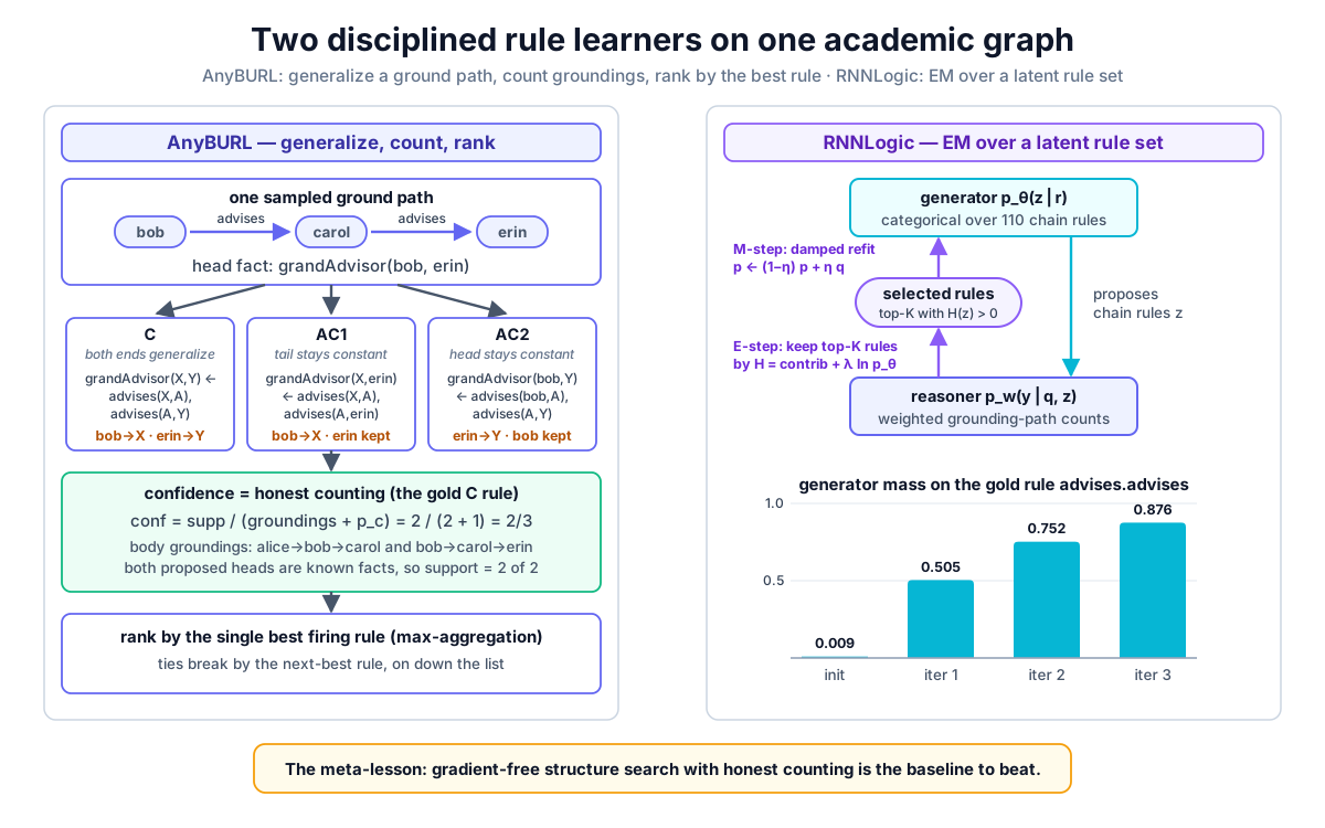Two disciplined answers to "which rules explain this graph": AnyBURL counts groundings of template-generalized paths and ranks by the best rule; RNNLogic treats the rule set as a latent variable and alternates rule selection with generator refitting. Original diagram by the authors, created with AI assistance.

Confidence is a counted ratio, with a thumb on the scale

Each mined rule gets one score, and the score is a ratio of counts. Two counts are needed. A body grounding of a rule is one assignment of entities to the rule's head variables under which the body chain holds on the observed graph; the support is the number of those groundings whose head atom is also a known fact. For a rule $R$, AnyBURL's confidence divides them, with one extra term [2]:

$$\mathrm{conf}(R) \;=\; \frac{\mathrm{supp}(R)}{\#\text{body groundings}(R) + p_c}.$$

The pessimism constant $p_c$ is a fixed positive number added to the denominator, a Laplace-style damping whose entire purpose is to distrust small samples: a rule seen to succeed once in one grounding should not score the same as a rule that succeeded a hundred times in a hundred. With $p_c = 1$, one-out-of-one scores $1/(1+1) = 0.5$ while a hypothetical hundred-out-of-a-hundred would score $100/101 \approx 0.99$; the damping vanishes as evidence accumulates. The published system uses $p_c = 5$, a fixed global setting, appropriate at a scale where useful rules have hundreds of groundings; the companion uses $p_c = 1$ (rule_mining.py line 72) because every support count on the toy graph is a single digit, and a damping of 5 would flatten the whole rulebook toward zero (the gold rule would score $2/7 \approx 0.286$ instead of $2/3$, and every support-1 rule would collapse to at most $1/6$). The constant's value is a knob; its presence is the principle. This way of scoring a rule descends from the ontology-mining tradition, where AMIE posed the sharper underlying question: what should the denominator even count when the graph is incomplete and a missing fact is not a false one [4]? AMIE's partial-completeness answer refines the denominator; AnyBURL keeps the simple closed-world count and lets $p_c$ absorb the distrust.

The companion computes the ratio exhaustively, template by template (rule_mining.py lines 170–197):

def confidence(rule: tuple) -> tuple[float, int, int]:
    """AnyBURL's sampled confidence, computed exhaustively here:

        conf(rule) = support / (#body groundings + pc)
    ..."""
    kind, head_rel, chain = rule[0], rule[1], rule[2]
    facts = HEAD_FACTS[head_rel]
    if kind == "C":
        # groundings: every (x, y) pair connected by the chain
        pairs = [(x, y) for x in kg.ENTITIES for y in chain_reach(x, chain)]
        support = sum((x, y) in facts for x, y in pairs)
        n_ground = len(pairs)

Now the worked count, done by hand for the gold rule grandAdvisor(X,Y) ← advises(X,A), advises(A,Y). The observed advises edges are alice → bob, bob → carol, carol → erin. Chains of two advises edges: (alice, bob, carol) and (bob, carol, erin), and no third, because erin advises nobody in the training set. So there are exactly 2 body groundings; note that on this graph every body-satisfying head pair has exactly one connecting chain, so counting chains and counting head-variable pairs (the definition above) give the same number, which is why the per-chain nested loop below is a valid independent check of the miner's per-pair count. The head pairs the two chains propose are (alice, carol) and (bob, erin), and both are derived grandAdvisor facts, so the support is 2:

$$\mathrm{conf} \;=\; \frac{2}{2 + 1} \;=\; \frac{2}{3} \;=\; 0.666\overline{6}.$$

This is not merely printed; it is asserted. The harness run() recomputes the two counts with an independent pair of nested loops over kg.TRAIN, code that shares nothing with the miner, and demands exact equality (rule_mining.py lines 361–374):

    ind_ground = ind_sup = 0
    for x, r1, a in kg.TRAIN:
        if r1 != "advises":
            continue
        for a2, r2, z in kg.TRAIN:
            if r2 == "advises" and a2 == a:
                ind_ground += 1                       # body: adv(x,a), adv(a,z)
                ind_sup += (x, z) in GOLD_GA          # head: grandAdvisor(x,z)
    gold_c = ("C",) + GOLD_RULE
    conf, sup, ng = mined[gold_c]
    assert (sup, ng) == (ind_sup, ind_ground) == (2, 2), \
        f"gold rule counts {(sup, ng)} != hand count {(ind_sup, ind_ground)}"

A second assert (lines 376–377) checks that this rule tops the confidence ranking of everything the miner found. The committed rulebook confirms both, with the gold rule at the top of the 14 rules that survive the support ≥ 1 gate:

[3] the mined rulebook (14 rules with support >= 1; conf = support/(groundings + 1))
      conf   sup/gnd   rule
     0.667   2/2       grandAdvisor(X,Y) <- advises.advises
     0.500   1/1       affiliated(X,mit) <- advises.affiliated
     0.500   1/1       grandAdvisor(X,carol) <- advises.advises
     0.500   1/1       grandAdvisor(X,erin) <- advises.advises
     0.500   1/1       affiliated(alice,Y) <- advises.affiliated
     0.500   1/1       affiliated(bob,Y) <- inv_advises.affiliated
     0.500   1/1       grandAdvisor(alice,Y) <- advises.advises
     0.500   1/1       grandAdvisor(bob,Y) <- advises.advises
    gold chain rule conf = 0.666667 == hand-counted 2/(2+1) (asserted, and the top rule overall)

Read the rulebook as a sociology of the graph. The general law sits on top. Beneath it, its own AC1/AC2 specializations each score 0.5 (one grounding, one success, damped), and genuinely useful side-knowledge appears: affiliated(X,Y) ← advises(X,A), affiliated(A,Y), "your student's institution is yours", mined at confidence 1/3, and its inverse reading "your advisor's institution is yours" at 1/4. At the bottom sits a spurious colleague heuristic, advises(X,Y) ← affiliated(X,A), inv_affiliated(A,Y), "you advise whoever shares your institution", correctly demoted to $1/(8+1) = 0.111$ because its body has 8 groundings and only one of them is a true advising pair. Counting, not gradients, sorted these.

Inference by maximum, and the ghost that returns for noisy-or

A mined rulebook ranks candidate edges as follows: a rule fires on a candidate (h, r, t) if its head relation is r and its body chain leads h to t (with AC constants matching), and each candidate is scored by aggregating the confidences of its fired rules. AnyBURL's choice is max-aggregation: score by the best fired rule, and break ties by the second best, then the next, and so on down the list until some rule separates the candidates [2]. The companion encodes the comparison as a zero-padded 3-tuple, which Python compares lexicographically for free (rule_mining.py lines 251–259); truncating the paper's unbounded tie-break at three components is the companion's simplification, and it is exact on this graph because no candidate fires more than two rules (the multi-fire audit at lines 399–412 finds a single two-rule candidate and nothing deeper):

def make_max_scorer(mined: dict):
    """AnyBURL's ranking: order candidates by best rule confidence, break
    ties by the next-best rule (lexicographic) — encoded as a 3-tuple score,
    zero-padded, which Python compares exactly lexicographically."""
    def score(h: str, r: str, t: str) -> tuple[float, float, float]:
        c = fired_confs(mined, h, r, t)
        return (c[0] if c else 0.0, c[1] if len(c) > 1 else 0.0,
                c[2] if len(c) > 2 else 0.0)
    return score

The natural-seeming alternative treats each fired rule as independent evidence and combines by noisy-or: if rules with confidences $c_1, \ldots, c_k$ fire, the candidate scores $1 - \prod_{i=1}^{k}(1 - c_i)$, the probability that "at least one rule is right" if the rules were independent coins (the product symbol $\prod$ multiplies the $k$ failure probabilities). Part II already met this fallacy under another name: computing the probability of a disjunction by multiplying failure probabilities is exactly the disjoint-sum error, valid only when the disjuncts are independent, and fired rules are anything but independent, because many are minor variants of one another that succeed and fail on the same groundings. Max-aggregation refuses the double count by construction, and the published finding is that it also ranks better in practice [2].

The committed run compares both, plus the frozen random baseline, on the six filtered ranking queries of the three held-out edges (kg.evaluate, kg.py lines 110–122):

[4] ranking the 3 held-out edges (filtered ranks: tail, head)
      test edge                     max      noisy-or  random
      (bob, advises, dave)          [3, 3]   [3, 3]    [8, 8]
      (bob, authored, p1)           [1, 1]   [1, 1]    [3, 2]
      (erin, affiliated, cmu)       [1, 2]   [1, 2]    [13, 10]
      filtered MRR                  0.6944   0.6944    0.21

The mean reciprocal rank (MRR), the average of one-over-rank across the queries, is worth one line of arithmetic for the max column: the six ranks are 3, 3, 1, 1, 1, 2, so $\mathrm{MRR} = \tfrac{1}{6}\left(\tfrac13 + \tfrac13 + 1 + 1 + 1 + \tfrac12\right) = \tfrac{1}{6} \cdot \tfrac{25}{6} = 0.6944$, more than three times the random baseline's 0.21, and the harness asserts the margin (rule_mining.py lines 383–384). Now the honest reading, which the module itself prints. The perfect ranks on (bob, authored, p1) are not knowledge: no mined rule fires for the relation authored at all, every candidate scores the zero tuple, and the filtered protocol's tie convention (ties resolve in the true entity's favour, kg.py lines 88–90) hands rank 1 to the true answer. The rank-1 on (erin, affiliated, cmu) is knowledge: the mined rule "your advisor's institution is yours" fires through erin's advisor carol, who is at cmu. And (bob, advises, dave) lands at rank 3 because in each direction two candidates, lifted by the spurious colleague-heuristic rules, outscore the unfired truth.

The max and noisy-or columns are identical, and it would be dishonest to read that as "aggregation does not matter." The module derives why they tie here rather than asserting it (rule_mining.py lines 391–412): on any candidate hit by exactly one rule, $1 - (1 - c) = c$, so noisy-or equals max, and the two scorers can only disagree on candidates hit by two or more rules. The harness enumerates the exact candidate set the protocol scores, 71 filtered candidates across the six queries, and finds exactly one multi-fire candidate: (bob, advises, bob), hit by the colleague heuristic at $c_1 = 1/3$ (its AC1 form) and $c_2 = 1/9$ (its C form). For that candidate,

$$1 - (1 - c_1)(1 - c_2) \;=\; 1 - \tfrac{2}{3} \cdot \tfrac{8}{9} \;=\; 1 - \tfrac{16}{27} \;=\; \tfrac{11}{27} \;\approx\; 0.4074 \;>\; 0.3333 = \max(c_1, c_2),$$

a strict boost (asserted at lines 410–411), and a textbook double count: the AC1 rule is a specialization of the C rule, so the two are perfectly correlated evidence, yet noisy-or treats them as independent witnesses. Here the boost lifted a candidate that was already ranked above the truth, so no rank moved; on real graphs, where a popular candidate can be hit by dozens of correlated rules, the same mechanism systematically inflates wrong answers, and that is the field's reported reason max-aggregation wins [2]. It is also, at benchmark scale, part of why rule-based systems as a family remain competitive with the entire embedding zoo: the comparative literature that ranks all these systems side by side keeps finding the counted-and-maxed baselines in the leading pack [3].

The anytime loop, and what the miniature keeps

The published system earns the "anytime" in its name with a control loop the toy does not need but the reader should know [2]. Mining proceeds in fixed time slices (one second each in the paper's configuration): each slice samples ground paths of the current length and generalizes them; after each slice the miner measures saturation, the fraction of sampled rules it had already seen, and when saturation crosses a threshold it concludes the current path length is exhausted and increases the length by one. A quality gate (in the paper, a rule must make at least two correct predictions) keeps junk out of the rulebook, and the whole process can be stopped at any moment, hence anytime: whatever rulebook exists when the clock runs out is usable, and more time only refines it. The miniature keeps the three templates, the damped confidence, and max-ranking, and drops the time boxing in favour of exhaustive enumeration; the module docstring states the trade explicitly (rule_mining.py lines 26–31), and nothing in the kept mathematics depends on it.

RNNLogic: the rule set as a latent variable

RNNLogic occupies the midpoint between AnyBURL's pure counting and the fully differentiable learners: the rules stay discrete, but which rules to use becomes a statistical inference problem [1]. Fix a query $q = (h, r, ?)$, asking for the entities related to head $h$ by relation $r$. Let $z$ denote a set of chain rules for relation $r$; $z$ is the latent variable, unobserved and to be inferred. Two models share the work. The generator $p_\theta(z \mid r)$, with parameters $\theta$, proposes rule sets for the query relation; in the published system it is a recurrent neural network (RNN, the network family that gives RNNLogic its name) emitting each rule as a sequence of relation tokens. The reasoner $p_w(y \mid q, z)$, with parameters $w$, scores each candidate answer $y$ by the weighted count of grounding paths that the rules in $z$ provide from $h$ to $y$ on the graph. The probability of an answer marginalizes over the latent rule set, summing over every possible $z$:

$$p(y \mid q) \;=\; \sum_{z} p_\theta(z \mid r)\; p_w(y \mid q, z).$$

Training maximizes the likelihood of the true answers, and the sum over rule sets is intractable, which is precisely the situation expectation-maximization (EM) was built for: alternate between inferring the latent variable given the current models (the E-step) and refitting the models given the inferred latent variable (the M-step). RNNLogic's E-step identifies a small set of high-posterior rules, the ones that contribute most to getting the true answers right while being plausible under the generator's current distribution; its M-step then treats those selected rules as observed data and refits the generator to them by maximum likelihood [1]. The gradients live inside the two models' parameter updates, the reasoner's per-rule weights and the generator's refit, and never flow through the logic: rule grounding stays a discrete, non-differentiated computation.

The companion miniaturizes each piece and says so out loud (rule_mining.py lines 31–35 of the docstring). The rule space is every chain of length 1 or 2 over the 10 signed relations, $10 + 10^2 = 110$ candidate bodies for the target relation grandAdvisor (lines 288–289). The generator becomes an explicit categorical distribution over those 110 chains, initialized uniform at $1/110 \approx 0.009091$: this is the honest miniature of the recurrent generator, a lookup table where the paper has a network. The queries are the two derivable grandAdvisor heads, alice with gold answer carol, and bob with gold answer erin (lines 292–294). One notational shift comes with the miniature: the selected set is assembled one rule at a time, so from here on $z$ ranges over individual chain rules, the elements of the latent set, and $p_\theta(z)$ reads as the generator's categorical probability of that single rule.

The E-step scores every rule $z$ by a two-term criterion (lines 319–322):

$$H(z) \;=\; \underbrace{\mathrm{contrib}(z)}_{\text{data term}} \;+\; \lambda \,\underbrace{\ln p_\theta(z)}_{\text{prior term}},$$

and keeps the top $K = 4$ rules with $H(z) > 0$. Decode both terms. The data term measures how much the rule helps answer the queries: for each query, walk the rule's body chain from the query head and collect the reached entities; award $+1$ for each gold answer reached and charge $0.5$ for each wrong entity reached (lines 297–306):

def contribution(chain: tuple[str, ...]) -> float:
    """The E-step's data term: how much the rule helps answer the queries.
    Per query, +1 if the chain reaches a gold answer from the query head,
    minus WRONG_COST for every non-answer it also reaches:
        contrib(z) = sum_q [ |reach ∩ gold| - 0.5 |reach - gold| ]."""
    total = 0.0
    for h, gold in GA_QUERIES:
        reach = chain_reach(h, chain)
        total += len(reach & gold) - WRONG_COST * len(reach - gold)
    return total

The prior term $\lambda \ln p_\theta(z)$ is the log of the generator's current probability for the rule, weighted by a small constant $\lambda = 0.1$ (line 73): a rule the generator already believes in needs less evidence to be selected, which is exactly the posterior flavour of the published E-step, where the selection criterion combines the rule's contribution to the answer likelihood with its generator prior [1]. Keeping $\lambda$ small keeps the data in charge; the prior only breaks near-ties.

The M-step refits the generator on the selected rules. The maximum-likelihood estimate (MLE) of a categorical distribution given weighted observations is just the normalized weights, so the target distribution puts mass $q(z) = \max(\mathrm{contrib}(z), 0) / \sum_{z' \in \text{selected}} \max(\mathrm{contrib}(z'), 0)$ on each selected rule and zero elsewhere (this $q$ is a new symbol, the standard EM name for the target distribution; it is unrelated to the query $q$). The update is applied damped, with step $\eta = 0.5$ (lines 329–332):

$$p_{\text{new}}(z) \;=\; (1 - \eta)\, p_{\text{old}}(z) \;+\; \eta\, q(z),$$

a convex mixture of the old distribution and the MLE target. The damping is the miniature's stand-in for the real system's gradient training: an RNN generator trained by stochastic gradient steps moves toward the maximum-likelihood fit gradually rather than jumping to it, and the mixture reproduces that gradual motion in closed form. Finally the reasoner answers each query by a weighted vote: every selected rule adds its generator probability to every entity its chain reaches, and the argmax (the highest-vote entity) is the prediction (lines 335–342).

Three iterations, every number re-derived

The committed trace is short enough to check line by line:

[5] RNNLogic's EM: generator mass converging onto the gold rule
      iter   p_gen(advises.advises)   #selected   H(gold)   H(runner-up)   reasoner acc
      init   0.009091                -           -         -              -
      1      0.504545                1           1.5300    -0.4700        1.00
      2      0.752273                1           1.9316    -0.5394        1.00
      3      0.876136                1           1.9715    -0.6087        1.00
    E-step keeps top-4 rules with H > 0; M-step is the damped MLE (eta = 0.5).

Derive iteration 1 by hand. The gold rule's chain advises∘advises (the composition symbol ∘ reads "then": first an advises edge, then another), walked from alice, reaches exactly one entity, carol, which is the gold answer; walked from bob it reaches exactly erin, again gold. No wrong entity is reached, so $\mathrm{contrib} = 1 + 1 = 2$. The generator is still uniform, so the prior term is $\lambda \ln(1/110) = 0.1 \times (-4.70048) = -0.47005$, and

$$H(\text{gold}) \;=\; 2 - 0.47005 \;=\; 1.5300,$$

the printed value. The runner-up tells the other half of the story: the best non-gold score is $-0.4700$, which is $0 + 0.1 \ln(1/110)$, a rule whose chain reaches nothing (contribution exactly 0) carried by the uniform prior alone. Every rule that does reach entities from the query heads but reaches wrong ones scores below that: the single-hop chain (advises,) reaches bob from alice and carol from bob, both wrong, so $\mathrm{contrib} = -0.5 - 0.5 = -1$. Only the gold rule clears $H > 0$, so despite $K = 4$ the selection keeps exactly one rule (hence #selected = 1), the target distribution is $q(\text{gold}) = 2/2 = 1$, and the damped update gives

$$p_{\text{new}}(\text{gold}) \;=\; 0.5 \times 0.009091 + 0.5 \times 1 \;=\; 0.504545,$$

again the printed value. Iterations 2 and 3 repeat the pattern with a growing prior: $H(\text{gold}) = 2 + 0.1 \ln(0.504545) = 2 - 0.0684 = 1.9316$, then $2 + 0.1 \ln(0.752273) = 1.9715$; the mass updates $0.5 \times 0.504545 + 0.5 = 0.752273$ and $0.5 \times 0.752273 + 0.5 = 0.876136$. Meanwhile every unselected rule's mass halves each iteration, so the runner-up's score falls, $0.1 \ln(1/220) = -0.5394$, then $0.1 \ln(1/440) = -0.6087$: the rich get richer, the poor get poorer, and the fixed point of the update is all mass on the gold rule. The reasoner, voting with the selected rule, answers both queries correctly from iteration 1 onward. The harness asserts the whole shape of this trace, not just its endpoint: the gold rule's mass rises strictly monotonically from $1/110$, it tops the E-step ranking every iteration, it ends above majority mass $0.5$, and the reasoner's accuracy ends at 1 (rule_mining.py lines 414–423).

Read what made this easy, because the reading is the honest part. The latent structure is clean: exactly one rule in the 110-chain space has positive contribution, so the E-step's selection problem has one right answer and the EM loop cannot oscillate between competing explanations. And the contributions are computed from exact grounding counts on a fully enumerable graph. At real scale both comforts vanish: the rule space grows exponentially with rule length, many near-equivalent rules split the credit, and grounding counts must themselves be approximated. The released system's answer to the cold-start half of this problem is telling: before the EM loop starts, its generator is pre-trained on candidate rules mined bottom-up from the training graph, the same ground-path harvesting AnyBURL begins with, a practical warm start rather than part of the formal objective [1]; the statistical machinery is seeded by symbolic rule evidence, not by gradients.

The unsolved part

Close the Part's ledger with three debts both methods owe, stated without softening.

First, the confidences are not probabilities. AnyBURL's $2/3$ and RNNLogic's $0.876$ look like probabilities, add like scores, and are neither: the first is a grounding ratio under a sampling scheme, a pessimism constant, and a closed-world denominator that counts every unknown fact as false; the second is one categorical's mass under a particular damping schedule (halve $\eta$ and the same three iterations end at a different number with the same ranking). Neither number is calibrated, in the sense Volume 5 will make precise: nothing guarantees that among all edges scored $0.67$, about two-thirds are true. Rankings survive this; any downstream use that reads the score as a chance does not.

Second, rule redundancy defeats aggregation in both directions. The chapter's multi-fire candidate showed noisy-or double counting two rules that were literally specializations of each other; that is redundancy punished under independence-style aggregation. But max-aggregation errs the opposite way: ten genuinely diverse weak rules, each independently right two times in three, jointly constitute strong evidence that max flatly ignores, scoring the candidate as if only the best rule existed. The right aggregation would need to know which rules are correlated and how, which is a joint distribution over rule firings that neither method models. Every fix on offer, from AMIE-style denominator surgery [4] to learned per-rule weights [1], treats a symptom.

Third, the template language is a ceiling. Everything in this chapter, and everything in this Part, learns chain rules (plus AnyBURL's one-constant variants): body atoms threaded in a line from one head variable to the other. No chain expresses "X and Y coauthored two different papers" (a body with a branching join and an inequality), "X advises at least three students" (a counting quantifier), or Volume 2's disjointness axioms (negation). Neural-LP, DRUM, NTP with chain templates, RNNLogic, and AnyBURL all share this bias, which is exactly why the honest symbolic baseline can match the neural methods: on benchmarks whose regularities are mostly chains, everyone is searching the same small language, and the differentiable detour buys little. Whether gradient-based search ever pays for itself in a larger rule language, where enumeration and counting genuinely break down, is the open question this Part hands to the research frontier.

Why it matters

The meta-lesson is the chapter's title read backwards: before believing any differentiable rule learner, run the symbolic control. That is not rhetoric; it is the same experimental discipline Volume 2 used when the from-scratch reasoner was checked against an oracle, and Volume 3 used when every embedding model had to beat a frozen random scorer under the same protocol. Here the control is stronger than the treatments often are, and the comparative literature says this is the normal state of affairs on knowledge-graph completion, not an artifact of toy scale [3]. For the road ahead, both methods also mark out Volume 5's territory: their uncalibrated confidences are precisely the trust problem the frontier volume takes up, and their explicit rules are the currency of its faithfulness chapters, because a prediction backed by "advises∘advises, confidence 2/3, groundings listed" is an explanation a human can audit, which no embedding score ever was. Part IV ends, then, with its two pillars in balance: logic supplied the rule language and the counting semantics; learning supplied a way to search and to weight. What neither supplied yet is a way to answer a compositional query, and that changes the question entirely.

Key terms

• AnyBURL (Anytime Bottom-Up Rule Learning) — a gradient-free rule miner: sample ground paths, generalize each into rule templates, score by sampled confidence, rank candidate edges by their best firing rule; anytime because mining runs in time slices and can stop at any moment with a usable rulebook [2].
• Ground path / language bias — a concrete constant-only walk from a fact's head to its tail; the language bias is the fixed menu of generalizations (which constants become variables) the miner will consider.
• C / AC1 / AC2 templates — the three generalizations of a ground path in the companion: cyclic (both head arguments variable, bound through the body chain), acyclic with the tail kept constant, acyclic with the head kept constant. The AC1/AC2 labels are the companion's: the published taxonomy folds both one-constant shapes into one constant-ending acyclic type (modulo flipping relations to their inverses) and reserves its second acyclic type for bodies ending at a fresh dangling variable, a shape the companion drops.
• Confidence with pessimism constant — $\mathrm{conf}(R) = \mathrm{supp}(R) / (\#\text{body groundings} + p_c)$; the constant $p_c$ (5 in the published system, 1 in the companion) damps rules with tiny support, and the ratio is exact counting on the observed graph.
• Max-aggregation vs noisy-or — ranking a candidate by its best fired rule with lexicographic tie-breaks, versus $1 - \prod_i (1 - c_i)$; noisy-or double counts correlated rules, the rule-level return of Part II's disjoint-sum problem.
• RNNLogic — rules as a latent variable $z$: a generator $p_\theta(z \mid r)$ proposes chain rules, a reasoner scores answers by weighted grounding-path counts, and an EM loop alternates rule selection with generator refitting [1].
• E-step rule score — $H(z) = \mathrm{contrib}(z) + \lambda \ln p_\theta(z)$: the rule's measured contribution to correct answers plus a small log-prior; the top-$K$ rules with positive score are selected.
• Damped M-step — $p_{\text{new}} = (1 - \eta)\,p_{\text{old}} + \eta\, q$ with $q$ the maximum-likelihood categorical on the selected rules; the closed-form miniature of a gradient-trained generator's gradual motion.
• Symbolic control — the methodological principle this Part closes on: a neural method's claim is measured as its margin over a disciplined symbolic baseline run under the identical protocol.

Where this leads

Part IV learned rules that predict single edges. The next Part changes the question: given the query "which institutions employ someone who advises a student of alice", the answer is not one edge but the result of a multi-hop, branching computation over the graph, with existential variables to bind along the way. Query Embedding: The Computation DAG opens Part V by making that computation itself the object that gets embedded: each query becomes a directed acyclic graph of projections and intersections, executed in vector space, and the running example's academic world supplies the multi-hop queries whose ground-truth answers the geometry will be audited against. The discipline travels with us: Part V's neural query answerers will be measured against symbolic query execution, exactly as this chapter measured gradients against counting.

---

Companion code: examples/integration/rule_mining.py implements both systems end to end on Volume 3's split of the academic graph: the signed graph and the derived grandAdvisor target (lines 87–122), path enumeration and the three templates (lines 127–158 and 200–217), exhaustive confidence with the pessimism constant (lines 170–197), the max, noisy-or, and frozen-random scorers under kg.py's filtered protocol (lines 232–280), RNNLogic's rule space, contribution function, and damped EM loop (lines 288–348), and the harness whose asserts guard every claim in this chapter, including the independent hand count of the gold rule's confidence and the shape of the EM trace (lines 354–433). Run python3 examples/integration/rule_mining.py to reproduce every number byte for byte; the run ends with SUMMARY rule_mining: rules=14 gold_conf=0.6667 mrr_max=0.6944 mrr_noisyor=0.6944 mrr_random=0.2100 p_gold=0.8761 em_acc=1.00.