Neural-LP and DRUM: Learning Chain Rules

📍 Where we are: Part IV · Differentiable Rule Learning — Chapter 12. GPU-Native NeSy ran a known rule as one matrix product on tensor hardware; this chapter opens Part IV by making the choice of rule itself the thing gradient descent searches for.

Volume 1 wrote the rule grandAdvisor(X,Z) ← advises(X,Y) ∧ advises(Y,Z) by hand, and every chapter since has consumed rules somebody already knew. The previous chapter showed that once a rule is fixed, applying it is a matrix product. This chapter removes the "fixed." Neural-LP (neural logic programming) places a learnable probability distribution over which relation matrices to multiply at each reasoning step, so that the discrete search through the space of chain rules becomes a continuous optimization a gradient can descend [1]. We train it on the academic graph's grandAdvisor queries, watch it rediscover Volume 1's rule from data alone, and audit the recovery the only honest way: by extracting the rule as a symbol string and replaying it with no floating point in sight. The second half of the chapter is a controlled failure. A head that needs two independent rules defeats the architecture for a reason we can prove in three lines, and the low-rank repair of DRUM (Differentiable RUle Mining) fixes it in a committed side-by-side run [2].

The simple version

Imagine teaching a delivery courier a route you refuse to state out loud. At every intersection the courier carries a little dial over the possible turns: 60 percent left, 30 percent straight, 10 percent right. Each day the courier drives the blend of all routes at once, you grade only the final doorstep, and the grade nudges every dial. After enough days the dials saturate: 99.9 percent "follow the advising street, then follow it again." Now you can read the route off the dials as written directions, hand them to a courier with no dials at all, and check that they reach every doorstep the training ever graded. That last check matters, because a dial that hedges between two genuinely different routes produces directions that are a smeared average of both, correct for neither. The hedging dial is this chapter's rank-1 defect; giving the courier two independent sets of dials is DRUM's repair.

What this chapter covers

• The differentiable-search framing: write rules, mine them discretely, or learn them by gradient, and the two stakes of the third way: learned rules inherit the data's noise, and extracted rules must actually be the weights' behavior.
• From enumeration to attention: the TensorLog score with explicit rule enumeration, every index decoded, and the combinatorial wall attention amortizes.
• The Neural-LP recurrence, derived and unrolled: per-hop attention over 11 operators, memory attention over previous states, and a full T = 2 hand trace naming the support of every intermediate vector.
• Training and gradients: the clamped negative log-likelihood, every gradient of the attention-matmul (matrix-multiplication) chain worked by the chain rule, the finite-difference certificate, and the committed loss trace from 13.7083 down to 0.0020.
• Extraction as audit: trained attentions unrolled into per-body confidence products, advises∘advises extracted at 0.9990, and the assert that the extracted symbolic rule reproduces every training answer and transfers to a held-out fact.
• The rank-1 defect and DRUM's repair: a designed two-rule head, the outer-product proof that rank-1 attention must entangle independent rules, the derived loss floor 4 ln 4 ≈ 5.5452 against the measured 5.5474, and the rank-2 run recovering both rules at 0.999 each.
• Scale and limits: what the real systems add (LSTM controllers, inductive evaluation), what chain rules cannot express, and why extracted confidences are not calibrated probabilities.

Who writes the rules?

Three answers exist, and this Part exists because the first two are not enough. The first is a person: Volume 1's kb.py states the grandAdvisor rule at line 79, and everything it derives is exactly as trustworthy as the author's insight. The second is discrete search: the rule-mining tradition (AMIE, Association Rule Mining under Incomplete Evidence; AnyBURL, Anytime Bottom-Up Rule Learning; and their relatives), treated in full in RNNLogic and the Symbolic Baseline AnyBURL; auditable, but every candidate rule is scored separately, and the candidate space explodes with rule length. The third is this chapter's: relax the discrete choice of rule into a continuous one, so that a single gradient-descent run searches the whole rule space at once, every rule's score updated simultaneously by every training example [1].

The relaxation buys speed and end-to-end training, and it charges two tolls that frame everything below. First, a learned rule is only as good as the data that taught it: it inherits every bias and gap in the training queries, silently. Second, after training you do not have a rule, you have a tensor of attention weights, and reading a discrete rule out of them is an act of interpretation that can lie. A rule extracted from a model is only worth stating if the rule, applied symbolically, reproduces what the model actually does. This chapter therefore treats extraction fidelity as a first-class experimental claim, guarded by an assert. DRUM's contribution, in this framing, is the discovery that fidelity is a rank property of the architecture [2]: one attention chain can be faithful to one rule, and provably cannot be faithful to two.

From a fixed chain to a weighted superposition

Recall the substrate from the previous chapter. Each of the academic graph's 5 relations (about, advises, affiliated, authored, cites) becomes a TensorLog operator: a 0/1 adjacency matrix $M_r$ of size $13 \times 13$, where 13 is the number of entities, with $M_r[h, t] = 1$ exactly when the fact $(h, r, t)$ (head entity $h$, relation $r$, tail entity $t$) is asserted [3]. This chapter builds its operators from the 15 training edges only (neural_lp.py lines 86–95); the split itself, which holds out three edges, among them (bob, advises, dave), the one the transfer test at the end needs, is Volume 3's kg.py TEST list and its guard asserts (lines 65–74). A query entity $x$ becomes the one-hot row vector $v_x$, twelve zeros and a single 1 at $x$'s index, and right-multiplying by $M_r$ pushes mass one hop along $r$: the entry $(v_x M_r)[t] = \sum_h v_x[h]\, M_r[h,t]$ sums, over every head entity $h$, the mass at $h$ times the indicator of an $r$-edge from $h$ to $t$.

A fixed chain rule is then a fixed product: applying advises twice is $v_x M_{\text{advises}} M_{\text{advises}}$. To learn a rule, TensorLog-style systems first write the score of an answer $y$ for a query $x$ as a weighted sum over every candidate rule body [1]:

$$\mathrm{score}(y \mid x) \;=\; \Big( v_x \sum_{l} \alpha_l \prod_{k \in \beta_l} M_{R_k} \Big)\, v_y^{\top}.$$

Decode every symbol before using it. The index $l$ ranges over candidate rule bodies: each $l$ names one possible chain, and $\beta_l$ is that body's ordered sequence of relation choices, so $\prod_{k \in \beta_l} M_{R_k}$ multiplies the chosen relation matrices in body order (for the body "advises then advises," written advises∘advises, where the composition symbol ∘ reads as "then" and the committed output and the tables below print rule bodies in this form, the product is $M_{\text{advises}} M_{\text{advises}}$, and $v_x$ pushed through it lands on $x$'s grand-advisees). The scalar $\alpha_l \ge 0$ is body $l$'s learnable confidence, the only trained quantity, and the final factor $v_y^\top$ reads off the mass the weighted superposition of all chains delivers to the candidate answer $y$ (the superscript $\top$ is the transpose, turning the one-hot row into a column so the read-off is a dot product). Learning rules now means learning the vector $\alpha$: a rule "exists" to the degree its confidence is large.

The formula is honest about its own cost. The sum over $l$ ranges over every body, and bodies multiply. With $T$ the maximum rule length (the number of reasoning hops) and $K$ the operator vocabulary size, there are $K^T$ bodies of length exactly $T$. The module's vocabulary doubles each relation with its inverse $\mathrm{inv}\_r$ (the transpose $M_r^\top$, a hop traversing an edge backward), Neural-LP's standard preparation, and adds DRUM's identity operator $I$ (a hop that stays put, letting a rule be effectively shorter than $T$), so both heads share one vocabulary and our tiny graph already has $K = 5 + 5 + 1 = 11$ operators and $11^2 = 121$ two-hop bodies (neural_lp.py lines 98–107). On a real knowledge base the wall is immediate: FB15K, a benchmark with 1,345 relations, has $2 \times 1345 + 1 = 2691$ operators and $2691^3 \approx 1.9 \times 10^{10}$ three-hop bodies, far too many to hold one $\alpha_l$ each [1]. The move that makes the problem tractable is to stop parameterizing bodies and start parameterizing hops.

The Neural-LP recurrence: attention over operators, attention over memory

Neural-LP replaces the $K^T$ body confidences with $T$ attention distributions over operators: at hop $t$ (from here on the letter $t$ counts hops, no longer a tail entity), a softmax vector $a_t$ of length $K$ says how much each operator participates in that hop [1]. Softmax turns $K$ raw scores into a distribution by exponentiating each score and dividing by the sum of the exponentials, so the $K$ entries are strictly positive and total 1; Volume 3's attention chapter derived its calculus, and its Jacobian returns in the gradient section below. A second device handles rules of different lengths: a softmax memory attention $b_t$ over all previous states chooses what each hop acts on, so a later hop can reach past intermediate results back to the raw query. One recurrence holds both:

$$u_t \;=\; \sum_{k=1}^{K} a_t[k] \; \Big( \sum_{\tau = 0}^{t-1} b_t[\tau]\, u_\tau \Big) M_k ,$$

where $u_0 = v_x$ is the one-hot query vector, $u_\tau$ the state after hop $\tau$ (a length-13 vector of soft mass over entities), and $t$ runs from 1 to $T$. Read it inside out: the memory attention $b_t$ blends all previous states into one vector, each operator $M_k$ pushes that blend one hop, and the operator attention $a_t$ blends the $K$ pushed results. A final read-out attention over $(u_0, \ldots, u_T)$ produces the prediction $p$. The companion module implements exactly this at $T = 2$ (neural_lp.py lines 183–202):

def nlp_forward(params: dict, x_id: int) -> tuple[np.ndarray, dict]:
    """The T = 2 Neural-LP recurrence  u_t = Σ_k a_t[k] · c_t M_k  with
    memory  c_t = Σ_{τ<t} b_t[τ] u_τ,  read out by  p = Σ_τ b_3[τ] u_τ.
    Returns (p, cache-for-backprop)."""
    u0 = np.zeros(N_E)
    u0[x_id] = 1.0
    a1, a2 = softmax(params["A"][0]), softmax(params["A"][1])
    b2, b3 = softmax(params["B2"]), softmax(params["B3"])
    # Step 1 (memory attention over {u_0} is the constant 1):  u_1 = Σ_k a_1[k] u_0 M_k.
    Y1 = apply_ops(u0)              # Y1[k] = u_0 M_k
    u1 = a1 @ Y1
    # Step 2 memory:  c_2 = b_2[0] u_0 + b_2[1] u_1.
    c2 = b2[0] * u0 + b2[1] * u1
    # Step 2:  u_2 = Σ_k a_2[k] c_2 M_k.
    Y2 = apply_ops(c2)              # Y2[k] = c_2 M_k
    u2 = a2 @ Y2
    # Final read:  p = b_3[0] u_0 + b_3[1] u_1 + b_3[2] u_2.
    p = b3[0] * u0 + b3[1] * u1 + b3[2] * u2
    return p, {"u0": u0, "u1": u1, "u2": u2, "c2": c2, "Y1": Y1, "Y2": Y2,
               "a1": a1, "a2": a2, "b2": b2, "b3": b3}

Note what the memory buys. If the read-out $b_3$ concentrates on $u_1$, the head answers with a one-hop rule; if hop 2's memory $b_2$ concentrates on $u_0$, hop 2 acts directly on the query and $u_2$ carries another one-hop rule; and the identity operator offers a third route to short rules by making a hop a no-op. Variable-length chain rules all live inside one fixed-depth computation, which lets a single gradient reach them all.

One honesty note before training, quoted from the module's header (neural_lp.py lines 34–44), because the published system has components this miniature deliberately drops; the LSTM (long short-term memory) and BiLSTM (bidirectional LSTM) controllers the quote mentions are the recurrent networks that emit the attentions in the full systems, and its logit tables are tables of raw pre-softmax scores:

Simplifications vs the real systems, stated plainly: the LSTM / BiLSTM
controllers that emit the attentions are replaced by directly-learned logit
tables (each head here trains a single query relation, so the controller's
output collapses to one table per hop — the recurrence would be dead
weight); operators are dense 13x13 NumPy arrays, not sparse tensors; plain
gradient descent replaces Adam with gradient clipping; T = 2 with no
validation split or early stopping; DRUM's per-step L1 normalization is
omitted (softmax attentions already keep mass bounded on this graph).  All
gradients are hand-derived (softmax Jacobian + chain rule through the
matmuls, in comments above the code) and verified against central finite
differences inside run().

In the full system one recurrent controller network emits $a_t$ and $b_t$ as a function of the query relation, so a single parameter set serves every relation at once [1]. Here each head trains one query relation, so the controller's output would be a constant per hop anyway; the module learns those constants directly as logit tables $A$, $B_2$, $B_3$, the raw pre-softmax scores the training actually updates (neural_lp.py lines 173–181), and says so.

Now the promised hand unroll, at the parameter setting training will be shown to approach: $a_1$ and $a_2$ one-hot on advises, $b_2 = (0, 1)$ (hop 2 reads $u_1$), $b_3 = (0, 0, 1)$ (the read-out takes $u_2$). The training graph's advises edges are alice→bob, bob→carol, carol→erin. Query alice: $u_0$ is one-hot on alice; hop 1 gives $u_1 = u_0 M_{\text{advises}}$, support exactly the set of people alice advises, so $u_1$ is one-hot on bob; the memory blend is $c_2 = u_1$; hop 2 gives $u_2 = c_2 M_{\text{advises}}$, one-hot on carol; the read-out returns $p = u_2$, all mass on carol. Query bob runs the same wiring through bob→carol→erin and puts all mass on erin. Those are precisely the training targets, computed by importing Volume 1's forward chainer (least_fixpoint, forward_chain.py lines 52–63) and collecting its derived grandAdvisor atoms over the same 15 training edges (neural_lp.py lines 124–144): alice → carol, bob → erin. The discrete rule is one corner of the continuous parameter space; the question is whether gradient descent walks there.

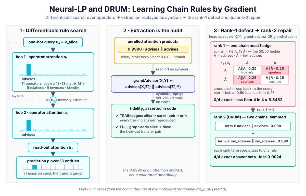Neural-LP makes the choice of rule differentiable (left), extraction replays the learned rule symbolically to prove fidelity (center), and the two-rule head shows rank-1 attention entangling what DRUM's rank-2 sum separates (right). Original diagram by the authors, created with AI assistance.

Training through the recurrence: the loss, the gradients, the trace

Each training query is a pair: a query entity $x$ and a multi-hot target vector $t$, with $t_y = 1$ for every true answer $y$ (this $t$ is a vector indexed by candidate answers, not the hop index of the recurrence). The loss is the negative log-likelihood the original system uses [1], with one defensive clamp (neural_lp.py lines 161–168):

$$L \;=\; -\sum_{y} t_y \, \log\!\big( \max(p_y, \varepsilon) \big), \qquad \varepsilon = 10^{-20}.$$

The clamp guards the general case, not this run. A target entity with no mass-carrying path from the query $x$ would receive exactly zero mass; $\log 0$ is negative infinity, and the derivative $\partial(-\log p)/\partial p$ (the symbol $\partial$ marks a partial derivative: the rate of change with respect to one variable while all others are held fixed) equals $-1/p$ and diverges. Clamping keeps the loss finite, and because $\max(p_y, \varepsilon)$ is constant for $p_y \le \varepsilon$, the gradient there is defined to be zero: the flat region contributes nothing, and learning is driven by the answers that already receive some mass. On this graph the clamp never fires: softmax entries are strictly positive, every training target is reachable through the advises hops, and the first-epoch loss of 13.7083 below confirms it, because a single clamped target would by itself contribute $-\ln 10^{-20} \approx 46$ to the loss, and a total of 13.71 leaves no room for one. Differentiating the unclamped region term by term, $\partial L / \partial p_y = -t_y / p_y$, which is exactly what _nll_grad returns.

From $\partial L / \partial p$ the chain rule walks the forward pass backward, and every step is one of two patterns. The linear blends are immediate: from $p = b_3[0]\, u_0 + b_3[1]\, u_1 + b_3[2]\, u_2$, the read-out weights get $\partial L / \partial b_3[\tau] = g_p \cdot u_\tau$ (write $g_p$ for $\partial L/\partial p$; nudging $b_3[\tau]$ adds $u_\tau$ to $p$, so the loss moves at rate $g_p \cdot u_\tau$), and each state receives its share, for instance $\partial L / \partial u_2 = b_3[2]\, g_p$. The attended matrix product (the "matmul") is the pattern worth deriving once in coordinates. Hop 2 computes entry $j$ of $u_2$ (the index letters $i$ and $j$ both range over the 13 entities, $i$ naming an entry of $c_2$ and $j$ an entry of $u_2$): $u_2[j] = \sum_k a_2[k] \sum_i c_2[i]\, M_k[i,j]$. Differentiate with respect to one attention weight:

$$\frac{\partial u_2[j]}{\partial a_2[k]} \;=\; \sum_i c_2[i]\, M_k[i,j] \;=\; (c_2 M_k)[j] \quad\Longrightarrow\quad \frac{\partial L}{\partial a_2[k]} \;=\; g_{u_2} \cdot (c_2 M_k),$$

the dot product of the upstream gradient with the $k$-th pushed image, which the forward pass already cached as $Y_2[k]$. Differentiate instead with respect to the state being pushed:

$$\frac{\partial u_2[j]}{\partial c_2[i]} \;=\; \sum_k a_2[k]\, M_k[i,j] \quad\Longrightarrow\quad \frac{\partial L}{\partial c_2[i]} \;=\; \sum_k a_2[k] \sum_j g_{u_2}[j]\, M_k[i,j] \;=\; \sum_k a_2[k]\, \big(g_{u_2} M_k^\top\big)[i],$$

the attention-weighted pull of the gradient backward through each operator's transpose (apply_ops_T, neural_lp.py lines 116–119). One state has two consumers and its gradients add: $u_1$ feeds both the read-out and hop 2's memory, so $\partial L/\partial u_1 = b_3[1]\, g_p + b_2[1]\, g_{c_2}$ (neural_lp.py lines 224–228). Finally every attention vector is a softmax of its logits (write $z$ for the logit vector and $s = \mathrm{softmax}(z)$ for its output), and Attention: Reasoning by Relevance derived the softmax Jacobian $\partial s_j / \partial z_i = s_j(\delta_{ij} - s_i)$ in Volume 3; contracting it with an upstream gradient $g$ gives

$$\frac{\partial L}{\partial z_i} \;=\; \sum_j g_j\, s_j (\delta_{ij} - s_i) \;=\; g_i s_i - s_i \sum_j g_j s_j \;=\; s_i \big( g_i - g \cdot s \big),$$

where $\delta_{ij}$ is the Kronecker delta, 1 when $i = j$ and 0 otherwise, so the first sum keeps only its $j = i$ term. That closed form is softmax_grad (neural_lp.py lines 155–159); the full backward pass is nlp_loss_and_grads (lines 204–236), each derivation repeated in comments above its line. None of this is taken on faith. Write $\theta$ for the stacked trainable logits (the tables $A$, $B_2$, $B_3$) and $h$ for the small probe step of a finite difference (a reuse of the letter, no longer the head-entity index; the code's parameter is literally named eps, set to $10^{-6}$): grad_check (lines 417–436) compares every hand-derived gradient entry against the central finite difference $(L(\theta + h) - L(\theta - h)) / 2h$, and the committed run certifies

[2] hand-derived gradients vs central finite differences (max rel err)
    Neural-LP head : 2.22e-09
    DRUM head      : rank-1 2.45e-09, rank-2 6.31e-09

Training is plain gradient descent, $\theta \leftarrow \theta - \eta\, \partial L / \partial \theta$, where $\eta$ is the learning rate, the step size of each update, set to $0.5$ for 3000 epochs (train_head, lines 238–251), on the two grandAdvisor queries. The committed trace:

[3] Neural LP on grandAdvisor(X, ?) — loss   L = −Σ_y t_y log max(p_y, 1e-20)
    epoch :  loss
        1 :   13.7083
       10 :    0.8102
      100 :    0.0617
     1000 :    0.0060
     3000 :    0.0020

The loss falls by a factor of almost 7000, and the module's competency check demands at least a 20-fold reduction before any further claim is allowed (neural_lp.py lines 489–490). But a low loss says only that the continuous model answers well. It does not yet say the model learned a rule.

Rule extraction is the audit

The extraction procedure inverts the recurrence. Every path through the computation graph is one chain rule, and its confidence is the product of the attention weights the path used [1]. At $T = 2$ there are exactly four path shapes (extract_rules, neural_lp.py lines 256–283):

read-out takes	hop-2 memory	body of the rule	confidence
$u_0$	—	$()$, the identity chain	$b_3[0]$
$u_1$	—	$(k)$	$b_3[1] \cdot a_1[k]$
$u_2$	$u_0$	$(k_2)$	$b_3[2] \cdot b_2[0] \cdot a_2[k_2]$
$u_2$	$u_1$	$(k_1, k_2)$	$b_3[2] \cdot b_2[1] \cdot a_1[k_1] \cdot a_2[k_2]$

Identity operators are deleted from bodies (they are the skip), identical bodies merge by summing confidence, and anything below the threshold 0.01 is pruned. The committed run extracts exactly one rule:

[4] extracted rules (attention products ≥ 0.01, Algorithm 1)
    0.9990  grandAdvisor(X,Y) ← advises(X,Z1) ∧ advises(Z1,Y)

[5] symbolic replay of the top rule (no floats — set-valued hops)
    over TRAIN edges : alice → ['carol'], bob → ['erin']   == every training answer
    over FULL graph  : alice → ['carol', 'dave'], bob → ['erin']   == Volume 1's closure, incl. the transfer pair (alice, dave)

Volume 1's rule, recovered from data at confidence 0.9990, with no competitor surviving the threshold. The replay in block [5] is what makes the claim honest. apply_rule (neural_lp.py lines 296–313) applies the extracted body as pure set-valued hops, no floating point anywhere, and the harness asserts two things (lines 497–502). First, fidelity: over the training edges, the symbolic rule reproduces every training answer exactly, so the extracted symbols really are the trained weights' behavior, not a story told about them. Second, transfer: on the full 18-edge graph, the rule derives grandAdvisor(alice, dave), a fact no training target contained, because it needs the held-out edge (bob, advises, dave). The rule generalizes for the structural reason rules always do: it mentions relations, not entities, so new edges flow through it for free. This is the inductive advantage the family claims over Volume 3's embedding models, which have nothing to say about an entity or edge they never embedded [2].

State the general principle plainly, because the next section is its violation. Extraction reads the confidence of body $(k_1, k_2)$ off a product of per-hop attentions, so it is only meaningful when the model's behavior actually factorizes that way: when the continuous model is (near-)low-rank over rule space, its mass concentrated on few enough rules that per-hop products can represent them. One rule is the friendly case: the attentions saturate, the product is nearly one on one body, and fidelity holds. Two rules is where the factorization breaks.

The rank-1 defect, run rather than cited

The companion module designs the failure instead of describing it. A new head, acadLine, is defined to have two independent clean chain rules over the advising chain: your academic line is your grand-advisor or your grand-student (neural_lp.py lines 318–323):

# The designed head with TWO independent clean chain rules over the graph:
#   acadLine(X,Y) ← advises(X,Z) ∧ advises(Z,Y)           (two hops DOWN)
#   acadLine(X,Y) ← inv_advises(X,Z) ∧ inv_advises(Z,Y)   (two hops UP)
# i.e. grand-advisor OR grand-student along the advising chain.
DRUM_BODIES: tuple[tuple[str, ...], ...] = (("advises", "advises"),
                                            ("inv_advises", "inv_advises"))

The targets are those two bodies applied symbolically over the training edges: alice → carol and bob → erin (down the chain), carol → alice and erin → bob (up the chain). Now consider what any single attention chain can express. Write $A$ for the advises operator and $\bar{A}$ for its inverse inv_advises (the bar marks the reversed direction; the symbol $I$ stays reserved for the identity operator), and abbreviate the confidence the extraction assigns to the two-hop body $(k_1, k_2)$ as $C[k_1, k_2] = a_1[k_1] \cdot a_2[k_2]$. As a matrix over operator pairs, $C = a_1 a_2^\top$ is an outer product, hence a rank-1 matrix, and a rank-1 matrix cannot have two large diagonal entries with small off-diagonal ones. The proof is one line of algebra on the cross terms:

$$C[A, \bar{A}] \cdot C[\bar{A}, A] \;=\; \big(a_1[A]\, a_2[\bar{A}]\big)\big(a_1[\bar{A}]\, a_2[A]\big) \;=\; \big(a_1[A]\, a_2[A]\big)\big(a_1[\bar{A}]\, a_2[\bar{A}]\big) \;=\; C[A, A] \cdot C[\bar{A}, \bar{A}],$$

the same four factors regrouped. So if both true rules carry confidence at least $c$, the two spurious cross bodies satisfy $C[A,\bar{A}] \cdot C[\bar{A},A] \ge c^2$, and at least one of them carries confidence at least $c$ too. Wanting both rules forces wanting their cross products. This is the miniature of DRUM's Theorem 1, which proves the rank-1 formulation cannot represent two independent chain rules without assigning their cross-terms high confidence [2].

The forced compromise is even computable in closed form. From alice, only the body $(A, A)$ reaches the target carol, and from carol only $(\bar{A}, \bar{A})$ reaches alice, so with the attention mass split between $A$ and $\bar{A}$ (mass on any other operator reaches no target and only raises the loss) the loss over the four one-answer queries is $L = -2 \ln\!\big(a_1[A]\, a_2[A]\big) - 2 \ln\!\big(a_1[\bar{A}]\, a_2[\bar{A}]\big)$. Substitute the constraint $a_1[\bar{A}] = 1 - a_1[A]$ and set the derivative to zero: $-2/a_1[A] + 2/a_1[\bar{A}] = 0$, so $a_1[A] = a_1[\bar{A}] = \tfrac12$, and identically for $a_2$. The optimum is the 50/50 hedge $a_1 = a_2 = (\tfrac12, \tfrac12)$, every body at confidence $\tfrac14$, with loss floor

$$L^{\star} \;=\; -4 \ln \tfrac14 \;=\; 4 \ln 4 \;\approx\; 5.5452 .$$

The committed run lands within 0.0022 of that floor (0.04 percent above it) and exhibits every predicted symptom:

    loss     rank-1     rank-2
        1   19.4184   16.4044
       10    6.4025    1.6764
      100    5.6128    0.0774
     1000    5.5517    0.0073
     3000    5.5474    0.0024
    learned 2-hop chains (confidence = product of hop attentions):
      rank-1 term 0: advises∘advises 0.250 | advises∘inv_advises 0.250 | inv_advises∘advises 0.250 | inv_advises∘inv_advises 0.250
      rank-2 term 0: inv_advises∘inv_advises 0.999
      rank-2 term 1: advises∘advises 0.999

The rank-1 loss stalls at 5.5474 against the derived 5.5452 while the rank-2 loss falls to 0.0024, and the rank-1 extraction is exactly the entangled quadruple: four bodies at 0.250 each, two of them rules nobody asked for. The spurious bodies are not harmless noise. From bob, advises∘inv_advises runs bob → carol → bob (carol's advisor is bob) and inv_advises∘advises runs bob → alice → bob: both cross chains loop back to the query entity, their confidences add, and the rank-1 model puts mass 0.50 on bob being his own academic line against only 0.25 on the true answer erin. The committed per-query table shows the measured damage, a star marking every predicted answer set that differs from the symbolic truth:

    query   symbolic   rank-1 p(ans)                rank-2 p(ans)
    alice   ['carol']  alice:0.25 carol:0.25*       carol:1.00
    bob     ['erin']   bob:0.50 erin:0.25*          erin:1.00
    carol   ['alice']  alice:0.25 carol:0.50*       alice:1.00
    erin    ['bob']    bob:0.25 erin:0.25*          bob:1.00
    mean p(true answers): rank-1 0.2499   rank-2 0.9994
    exact answer sets   : rank-1 0/4        rank-2 4/4

The harness does not merely eyeball this: it asserts that the rank-1 spurious self-answer outscores the true answer for bob (neural_lp.py lines 513–516), that rank-1 wins strictly fewer exact answer sets than rank-2's asserted four (the printed run shows zero), and that the gaps in mean target mass and final loss are wide, not marginal (lines 503–511).

DRUM: the low-rank repair

DRUM's estimator drops the memory attention (the identity operator alone covers shorter rules) and instead runs $L$ independent attention chains, summing their results; the letter $L$ here is the rank, the number of chains [2]:

$$p \;=\; \sum_{j=1}^{L} v_x \prod_{t=1}^{T} \Big( \sum_{k=1}^{K} a_{j,t}[k]\, M_k \Big),$$

where $a_{j,t}$ is chain $j$'s operator attention at hop $t$. Expanding the product of sums for one chain, $\prod_t \big(\sum_k a_{j,t}[k] M_k\big) = \sum_{k_1, \ldots, k_T} \big(\prod_t a_{j,t}[k_t]\big) M_{k_1} \cdots M_{k_T}$: chain $j$ assigns body $(k_1, \ldots, k_T)$ the confidence $\prod_t a_{j,t}[k_t]$, an outer product of $T$ vectors, so the head's total confidence tensor is a sum of $L$ outer products. That is precisely a CP decomposition (canonical polyadic: a tensor written as a sum of rank-1 tensors), and DRUM's Theorem 2 is the matching sufficiency result: with enough rank, the estimator represents any finite weighted set of chain rules, each rank term free to specialize to one rule [2]. Rank 1 recovers exactly the entangled form above, which is why the module implements both as one function with a rank parameter (drum_forward, neural_lp.py lines 344–365):

    rank = params["A"].shape[0]
    u0 = np.zeros(N_E)
    u0[x_id] = 1.0
    a = np.stack([[softmax(params["A"][j, t]) for t in range(T)]
                  for j in range(rank)])          # (L, T, K) attentions
    us = np.zeros((rank, T + 1, N_E))             # u[j, t] = state of chain j
    ys = np.zeros((rank, T, K, N_E))              # ys[j, t, k] = u[j,t] M_k
    us[:, 0] = u0
    for j in range(rank):
        for t in range(T):
            # u_{j,t+1} = Σ_k a_{j,t}[k] · u_{j,t} M_k
            ys[j, t] = apply_ops(us[j, t])
            us[j, t + 1] = a[j, t] @ ys[j, t]
    # p = Σ_j u_{j,T}   (the CP sum over the L rank terms)
    p = us[:, T].sum(axis=0)

Backpropagation adds nothing new: the CP sum routes the loss gradient $\partial L / \partial p$ ($L$ the loss again here, not the rank) to every chain unchanged, and each chain reuses the attended-matmul gradients derived above (drum_loss_and_grads, lines 367–388; finite-difference-checked to 6.31e-09). One initialization detail matters, and the code comments on it (lines 337–342): the rank terms start from small random logits, because identical starts would receive identical gradients forever and never specialize. Trained at rank 2 on the same queries, the committed run above shows the clean separation: term 0 saturates on inv_advises∘inv_advises at 0.999, term 1 on advises∘advises at 0.999, and the harness asserts all four rank-2 answer sets equal the symbolic ground truth (lines 503–505). One architecture, one hyperparameter changed, and the summary line compresses the exhibit:

SUMMARY neural_lp: top_rule=advises∘advises conf=0.9990 nlp_loss=0.0020 drum_p_tgt_r1=0.2499 drum_p_tgt_r2=0.9994 exact_r1=0/4 exact_r2=4/4

metric (committed run)	rank-1	rank-2
final loss (epoch 3000)	5.5474 (floor $4\ln 4 \approx 5.5452$)	0.0024
learned chains ≥ 0.01	four bodies at 0.250 (two spurious)	advises∘advises 0.999; inv_advises∘inv_advises 0.999
mean mass on true answers	0.2499	0.9994
exact answer sets	0/4	4/4
worst symptom	bob's spurious self-answer at 0.50 outscores erin at 0.25	none asserted

Scale, controllers, and what a chain cannot say

The real systems scale this skeleton in three directions. First, the controller: Neural-LP emits its attentions from an LSTM (long short-term memory network) conditioned on the query, and DRUM uses bidirectional LSTMs, one per rank, so a single trained model serves every query relation and hop attentions can coordinate along the chain [1][2]. Second, the operator vocabulary: the inverse-relation doubling is kept, and the operators become sparse tensors, so a hop costs proportional to the edge count rather than the entity count squared (the previous chapter's sparsity economics). Third, and most consequential, the evaluation regime: because a learned chain rule mentions no entities, these models are natively inductive, and DRUM's evaluation makes the contrast explicit by testing on graphs whose entities never appeared in training, where rules keep working and entity-embedding methods have no vector to look up [2]. Volume 3 ended on exactly this vocabulary-dependence critique; differentiable rule learning answers it by construction.

The honest boundary of the family is its chain bias. Everything above searches bodies of the form $r_1(X, Z_1) \wedge r_2(Z_1, Z_2) \wedge \cdots$: a single path of fresh variables from $X$ to $Y$. Rules whose bodies branch (a tree: "X and Y wrote a paper together and share an institution"), compare siblings, or close a cycle are outside the searched space no matter the rank, because no sequence of matrix products expresses them. Widening the space is its own research line: the template-based tradition's flagship ∂ILP (differentiable inductive logic programming) allocates soft weights over instantiations of general clause templates rather than chains, buying branching bodies and recursion at a memory cost that confines it to far smaller domains [4], and the next chapters' provers and probabilistic-logic learners (the differentiable backward chaining of NTP, the Neural Theorem Prover; RNNLogic's generator-reasoner split) attack the same space from other angles. Chains are not the end of rule learning; they are the part of it that fits inside a matrix product.

The unsolved part

A softmax never outputs an exact one-hot vector: its entries are ratios of exponentials, all strictly positive, so the trained attention always spreads some mass over every operator. The extraction at 0.9990 rounds a haze away, and on this graph the haze is harmless. But the general gap is real and unresolved. The continuous model that answers queries is the full superposition, haze included; the extracted rule set is a thresholded portrait of it. Between them sits a fidelity gap that is measured, never guaranteed: our replay assert is an empirical check on one graph, not a theorem, and at scale the papers report the model's ranking metrics and present extracted rules for inspection; the two need not agree, and nothing forces a comparison. When they diverge, which one is "what the model learned"? Volume 5 returns to exactly this question for rule extraction from trained systems, with faithfulness as the headline criterion. A quieter problem rides along: the confidence 0.9990 is an attention product, a quantity the softmax geometry produces, not a calibrated probability that the rule holds with that frequency in the world. Treating extracted confidences as probabilities is unlicensed, and the calibration instruments that would license or refute such readings are also Volume 5's business.

Why it matters

This chapter closes a loop the series opened in its first volume. Volume 1 wrote a rule and executed it; Volume 3 learned representations but could not say what they meant; here, for the first time, learning produces a symbol: a rule that can be printed, inspected, debated, and executed by a reasoner that has never heard of gradients. That round trip, weights to symbols to verified behavior, is the neuro-symbolic promise in its most concrete form, and its discipline here (extraction replayed, fidelity asserted, failure exhibited on a designed case) is the standard every interpretability claim in Volume 5 will be held to. The rank analysis carries its own general lesson: whether a continuous relaxation can be trusted to mean its discrete reading is a property of the architecture's expressiveness, provable in both directions, not a matter of training luck. And the inductive behavior of learned rules, transferring to entities and edges never seen, is the capability the complex-query and foundation-model chapters ahead keep returning to.

Key terms

• TensorLog operator — a relation as a 0/1 adjacency matrix $M_r$; right-multiplying a mass vector pushes it one hop along $r$. The substrate both Neural-LP and DRUM search over.
• Chain rule (logical) — a Horn rule whose body is a single path of fresh variables, $r_1(X, Z_1) \wedge \cdots \wedge r_T(Z_{T-1}, Y)$; evaluable as an ordered matrix product, and this chapter's entire hypothesis space.
• Operator attention $a_t$ — the per-hop softmax over the 11 operators (5 relations, 5 inverses, identity), replacing the discrete relation choice with a differentiable blend.
• Memory attention $b_t$ — the softmax over previous states letting a hop act on any earlier result, so rules shorter than the unrolled depth $T$ live inside the same recurrence.
• Rule extraction — unrolling trained attentions into per-body confidence products (identity dropped, duplicates merged, small products pruned) to read a discrete rule set out of a continuous model.
• Extraction fidelity — the requirement that the extracted symbolic rule, applied with set-valued hops and no floats, reproduce the trained model's answers; asserted here, merely measured at scale.
• Rank-1 entanglement — a single chain's body confidences form the outer product $a_1 a_2^\top$, forcing $C[A,\bar{A}]\cdot C[\bar{A},A] = C[A,A]\cdot C[\bar{A},\bar{A}]$ (with $A$ the advises operator and $\bar{A}$ its inverse): two independent rules cannot both be confident without a confident spurious cross-term.
• CP decomposition / rank $L$ — the body-confidence tensor as a sum of $L$ outer products, one per independent attention chain; DRUM's repair, sufficient for any weighted set of $L$ chain rules.
• Inductive rule application — a learned rule mentions relations, not entities, so it transfers to held-out edges and unseen entities where entity-embedding models have nothing to look up.

Where this leads

Neural-LP and DRUM learn rules by making the rule body soft while the entities stay crisp: mass flows along real edges, and only the choice of relation is blurred. The next chapter, Neural Theorem Proving: NTP and CTP, blurs the other half. There, the prover keeps the discrete shape of backward chaining, goals, unification, substitution, but replaces symbol-equality with vector similarity, so that "advises unifies with mentors" becomes a matter of embedding distance and a proof succeeds to a degree. Where this chapter's models answered "which chain of known relations explains the data?", a neural theorem prover asks the stranger question underneath it: what should it even mean for two symbols to almost match?

---

Companion code: examples/integration/neural_lp.py implements this entire chapter: the operator vocabulary (lines 86–107), the Neural-LP recurrence and hand-derived backward pass (lines 149–251), extraction and symbolic replay (lines 256–313), the acadLine head with the rank-1 and rank-2 DRUM estimators (lines 316–402), the finite-difference certificate (lines 417–436), and the competency asserts guarding every claim quoted here (lines 487–516). Training targets come from Volume 1's forward chainer (examples/logic/forward_chain.py lines 52–63), never retyped; the fixed-rule substrate (relations as adjacency matrices) was the previous chapter's subject, examples/integration/tensor_ops.py, though this module rebuilds its own operators from the 15 TRAIN edges only. Run python3 examples/integration/neural_lp.py to reproduce every number byte for byte; the run ends with SUMMARY neural_lp: top_rule=advises∘advises conf=0.9990 nlp_loss=0.0020 drum_p_tgt_r1=0.2499 drum_p_tgt_r2=0.9994 exact_r1=0/4 exact_r2=4/4.