Many-Valued Logic: Beyond True and False

📍 Where we are: Part I · Fuzzy and Many-Valued Logic — Chapter 1. Volume 3 closed with The Honest Verdict: embeddings rank and retrieve, but they do not deduce. Volume 4 opens by rebuilding logic itself so that gradients can reach it, and the rebuild starts at the very bottom, with the truth values.

Every logic this series has used so far, the Horn rules of Volume 1, the EL++ reasoner of Volume 2, the entailment gold standards of Volume 3, ran on exactly two truth values. A fact held or it did not; a subsumption was entailed or it was not. This volume's project is to make logic differentiable, and a function on a two-point set has no useful derivative: there is nowhere to move. So the first, unavoidable step is to enlarge the set of truth values, and this chapter takes the smallest honest step possible. We add one value, a middle value written ½, define the connectives, and then watch very carefully what breaks. The answer is: more than you would guess, in ways that are decided by a single truth-table entry, and everything in this chapter is computed rather than asserted. The companion module examples/integration/many_valued.py builds both classical three-valued logics from their definitions, checks the computed tables entry by entry against independently hardcoded textbook tables, decides every tautology claim by exhaustive enumeration, and verifies the final bridge to the unit interval exactly, with equality asserts rather than tolerances.

The simple version

Imagine a courtroom that allows only two verdicts, guilty and not guilty. Some cases genuinely fit neither: the evidence is thin, the witness never arrived, the truth is simply not established either way. Scottish courts historically kept a third verdict, "not proven," for exactly this situation. Now imagine the court also has to combine verdicts: if charge A is proven and charge B is not proven, what is the verdict on "A and B"? You need rules for combining three verdicts instead of two, and it turns out there is more than one reasonable rulebook. The two rulebooks in this chapter agree about "and," "or," and "not," and disagree about exactly one line of the "if... then..." rule. That one line decides whether the court has any laws at all, statements it must accept no matter the evidence. And once you allow a verdict to be a number, "70 percent established," the rulebooks become formulas, and formulas can be differentiated. That is the door this whole volume walks through.

What this chapter covers

• The overflow: why two truth values already failed us twice, in Volume 2's open world (unknown is not false) and in Volume 2's annotated facts (a citation edge carrying confidence 0.5 is neither true nor false), and why the honest fix is to enlarge the truth set rather than round the middle away.
• Three values, one design decision: negation as $1-x$, conjunction as min, disjunction as max, read order-theoretically as meet and join on the truth order; the full 3×3 tables computed by the companion and checked against hardcoded textbook tables.
• The implication fork: Kleene's material reading $\max(1-x,\,y)$ versus Łukasiewicz's residual reading $\min(1,\,1-x+y)$; the two tables differ at exactly one entry, and that entry decides whether the logic has tautologies.
• Designated values, decoded: what "tautology" even means once there are three values, why the choice of which values count as asserted is a separate dial from the tables, and the exhaustive-enumeration machinery that decides each verdict.
• The drift table, run not stated: seven classical laws scored across classical logic, K3 (Kleene's strong three-valued logic), and Ł3 (Łukasiewicz's three-valued logic); K3 keeps none, Ł3 keeps four, and each failure comes with the exact valuation that sinks it.
• The bridge to the interval: the same three definitions read on all of $[0,1]$, the computed proof that Ł3's arrow is the Łukasiewicz residuum restricted to three points, and the truth-functionality caveat that separates degrees of truth from probabilities.
• The agenda this sets: once truth values live in $[0,1]$, every connective is a real-valued function on the unit square, and "does this logic have useful gradients" becomes a well-posed mathematical question, the exact business of the next two chapters.

Why two truth values run out

Volume 2 taught the open-world lesson the hard way: under the open-world assumption, a fact absent from the knowledge base is not false, merely unstated. When the academic world's knowledge base did not record whether Dave advises anyone, the honest answer to "does Dave advise someone?" was not "no" but "unknown." Classical two-valued logic has no way to hold that answer. Every proposition must be 0 or 1, so "unknown" gets rounded, silently, to one of them, and the rounding is a lie in one direction or the other.

The second overflow came from Volume 2's annotated reasoner, and it is quantitative rather than epistemic. The annotated knowledge base attaches a confidence, a number in the unit interval $[0,1]$ (all real numbers from 0 to 1 inclusive), to every fact: the citation edge cites(p3, p2) carries 0.9, cites(p2, p1) carries 0.8, and the direct edge cites(p3, p1) carries exactly 0.5. That last value is the perfect provocation: a fact that its own knowledge base rates as no more true than false. The companion module refuses to retype this running example; it imports the edge list straight from Volume 2's code (many_valued.py line 51) and reads the 0.5 back out (many_valued.py lines 258–264). The committed run opens with it:

[1] the third truth value is already in the running example
    Volume 2's CONFIDENCE semiring ([0,1], max, min) labels the
    direct edge cites(p3, p1) with 0.5 — neither true nor false.
    excluded middle on it: max(0.5, 1-0.5) = 0.5  (a classical LAW, now half-true)

Both overflows point the same way: the truth set is too small. The smallest possible enlargement adds one value halfway between the two, giving the three-element truth set $V_3 = \lbrace 0, \tfrac{1}{2}, 1 \rbrace$ (many_valued.py line 57). What should ½ mean? History supplies two answers, and the difference between them will turn out to be the whole plot of this chapter. The older reading, proposed in 1920 for statements about the contingent future ("there will be a sea battle tomorrow"), takes ½ as possible: not yet settled either way, but a genuine third status a proposition can occupy; the system built on this reading is now called Ł3, Łukasiewicz's three-valued logic [1]. The second reading, built two decades later for the theory of partial computable functions and given its textbook form in 1952, takes ½ as undefined or unknown: the proposition is really true or really false, we just cannot tell, perhaps because the computation that would decide it never halts; this reading's system is K3, Kleene's strong three-valued logic [2]. And Volume 2's confidences suggest a third reading that neither system intended: ½ as a degree, a graded amount of truth, the reading that fuzzy set theory would later extend across the entire interval [3]. Keep the three readings mentally separate. They share arithmetic but not philosophy, and the chapter's closing caveat turns on the distinction.

Three values, one design decision

Now the connectives. Rather than legislating three fresh truth tables, both historical systems derive everything from one design decision: respect the order. Read $0 \lt \tfrac{1}{2} \lt 1$ as an ordering of truth, "false below undecided below true." On an ordered set, two canonical operations are defined whenever they exist: the meet of two elements, their greatest lower bound, and the join, their least upper bound (on a general partial order, an ordering that may leave some pairs uncompared, a pair of elements may have neither; an order in which every pair has both is called a lattice). On a totally ordered set like $V_3$, one in which any two elements are comparable, they always exist and are simply the minimum and the maximum. Define conjunction as the meet and disjunction as the join: a conjunction is only as true as its weaker conjunct, a disjunction as true as its stronger disjunct. For negation, take the map that flips the order end for end while fixing the midpoint, which on numbers is $x \mapsto 1-x$ (the symbol $\mapsto$ reads "maps to"). Both systems adopt all three definitions unchanged; the companion implements them in three one-line functions and then defines the two rival implications beside them (many_valued.py lines 60–82):

def neg(x: float) -> float:
    # ¬x = 1 - x                      (strong negation; shared by K3 and Ł3)
    return 1.0 - x


def conj(x: float, y: float) -> float:
    # x ∧ y = min(x, y)               (shared by K3 and Ł3)
    return min(x, y)


def disj(x: float, y: float) -> float:
    # x ∨ y = max(x, y)               (shared by K3 and Ł3)
    return max(x, y)


def imp_k3(x: float, y: float) -> float:
    # K3 implication: x → y = ¬x ∨ y = max(1 - x, y)   (material implication)
    return max(1.0 - x, y)


def imp_l3(x: float, y: float) -> float:
    # Ł3 implication: x → y = min(1, 1 - x + y)        (Łukasiewicz residuum)
    return min(1.0, 1.0 - x + y)

The full truth tables are then not axioms to memorize but arithmetic to perform. The function truth_table (many_valued.py lines 98–100) evaluates each connective at all nine input pairs, and run() asserts every computed entry against a hardcoded transcription of the textbook tables (many_valued.py lines 90–95 and 194–198), a genuine two-source comparison: if the one-line definitions and the published tables disagreed anywhere, the module would refuse to run. Here are the two shared tables as the committed run prints them, rows indexed by $x$, columns by $y$:

    x ∧ y = min(x, y)          (both logics)
      x\y |  0   ½   1
      ----+------------
       0  |  0   0   0  
       ½  |  0   ½   ½  
       1  |  0   ½   1  
    x ∨ y = max(x, y)          (both logics)
      x\y |  0   ½   1
      ----+------------
       0  |  0   ½   1  
       ½  |  ½   ½   1  
       1  |  1   1   1  

Every entry is an instance of the min/max arithmetic. The middle cell of the conjunction table is $\tfrac{1}{2} \wedge \tfrac{1}{2} = \min(\tfrac{1}{2}, \tfrac{1}{2}) = \tfrac{1}{2}$: two half-established claims conjoin to a half-established claim. The corner cells reproduce classical logic exactly, because on the subset $\lbrace 0, 1 \rbrace$ the minimum is the Boolean AND and the maximum is the Boolean OR. That containment is worth pausing on: both three-valued systems extend the classical tables conservatively at the level of the connectives, in the sense that restricting any connective to classical inputs returns classical outputs. (This is a property of the tables, not of the logics as theories; which laws survive is a very different question, as the drift table below will show.) Whatever breaks in three-valued logic will not break because the old cases changed; it will break because the new value ½ flows through the old laws in ways two-valued reasoning never had to survive.

Notice also what negation does to the middle value: $\neg \tfrac{1}{2} = 1 - \tfrac{1}{2} = \tfrac{1}{2}$. The midpoint is a fixed point of negation, the only truth value that is its own opposite. That single identity is the engine behind the famous failure in the run's opening lines: the law of the excluded middle, $p \vee \neg p$ (the letter $p$ is a propositional variable, a name for any proposition whose truth value can be set freely), classically a tautology, evaluates at $p = \tfrac{1}{2}$ to

$$\tfrac{1}{2} \vee \neg\tfrac{1}{2} \;=\; \max\!\big(\tfrac{1}{2},\; 1 - \tfrac{1}{2}\big) \;=\; \max\!\big(\tfrac{1}{2}, \tfrac{1}{2}\big) \;=\; \tfrac{1}{2},$$

which is exactly the "excluded middle on it: 0.5" line printed against the running example's half-confidence citation edge. A classical law, now half-true. Whether that outcome is a scandal or merely honest bookkeeping depends on what ½ means, and on one more definition we have not yet made: which truth values count as asserted. Both questions come to a head at the implication.

Implication is where the systems part

Classically, $p \rightarrow q$ (with $q$ a second propositional variable) can be defined away as $\neg p \vee q$: an implication is true unless its antecedent is true and its consequent false. K3 keeps that material reading verbatim, substituting the three-valued connectives (in the display below, the symbol $:=$ reads "is defined as") [2]:

$$x \rightarrow_{K3} y \;:=\; \neg x \vee y \;=\; \max(1 - x,\; y).$$

Ł3 instead defines the arrow directly, by a formula whose deeper justification (it is a residuum, an "inverse" of conjunction in a precise sense we compute at the end of this chapter) had to wait decades for the algebraic machinery to name it [1]:

$$x \rightarrow_{Ł3} y \;:=\; \min(1,\; 1 - x + y).$$

How different are they? The companion computes both 3×3 tables and then searches all nine input pairs for disagreements; the assert demands that the list of differing entries be exactly one pair long (many_valued.py lines 199–202). The committed run prints both tables with the disagreement starred:

    x → y = max(1-x, y)        (K3)
      x\y |  0   ½   1
      ----+------------
       0  |  1   1   1  
       ½  |  ½   ½*  1  
       1  |  0   ½   1  
    x → y = min(1, 1-x+y)      (Ł3)
      x\y |  0   ½   1
      ----+------------
       0  |  1   1   1  
       ½  |  ½   1*  1  
       1  |  0   ½   1  
    disagreement entries: (½, ½)  →  K3 gives ½, Ł3 gives 1

Eight of nine entries agree. The single divergence sits at $(x, y) = (\tfrac{1}{2}, \tfrac{1}{2})$, and it is worth computing both sides by hand, because the entire tautology story downstream hangs on this one cell. Under K3:

$$\tfrac{1}{2} \rightarrow_{K3} \tfrac{1}{2} \;=\; \max\!\big(1 - \tfrac{1}{2},\; \tfrac{1}{2}\big) \;=\; \max\!\big(\tfrac{1}{2},\; \tfrac{1}{2}\big) \;=\; \tfrac{1}{2}.$$

Under Ł3:

$$\tfrac{1}{2} \rightarrow_{Ł3} \tfrac{1}{2} \;=\; \min\!\big(1,\; 1 - \tfrac{1}{2} + \tfrac{1}{2}\big) \;=\; \min(1,\; 1) \;=\; 1.$$

Read the two verdicts through their intended readings and both make sense. K3's ½ means "unknown," and the honest defense of its verdict is mechanical rather than epistemic. K3 is truth-functional: by construction, the value a compound receives must be a function of the values its parts receive, so once both parts sit at ½ the arrow can return only what its table holds at (½, ½), whatever the formula's shape. What it cannot express is "true in every completion of the unknown," even though that stronger claim is available here: if $p$ is really 0 or really 1, then "$p$ implies $p$" comes out true either way, and a reasoner that quantified over all completions, asking whether the formula comes out true however the unknowns are resolved, would certify it, at the price of no longer computing compounds from their parts. Truth-functional bookkeeping for ignorance is local and cheap, and its cost is that even "$p$ implies $p$" goes unscored. Ł3's ½ means "possible," and its arrow measures something else entirely: how far the consequent falls short of the antecedent. In the formula $\min(1, 1 - x + y)$, the quantity $x - y$ is the shortfall, the amount of truth lost crossing the arrow; the implication is fully true whenever $y \ge x$, and is docked exactly the shortfall otherwise, since for $y \lt x$ the value is $1 - (x - y)$. An implication from a claim to itself has zero shortfall, so it is perfectly true, whatever the claim's status. One reading preserves ignorance; the other measures degradation. Both are coherent. They cannot both be your logic.

On classical inputs the fork disappears: for $x, y \in \lbrace 0, 1 \rbrace$ the two formulas agree everywhere, which the module also asserts (many_valued.py lines 205–207); the symbol $\in$ reads "is an element of." So the disagreement is invisible to any two-valued test and surfaces only when ½ actually flows through the arrow. To see what it decides, we need the chapter's central definition.

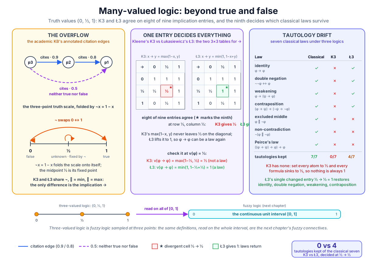One truth-table entry, the implication at (½, ½), separates a logic with no tautologies from a logic with four of the classical seven; the same three definitions, read on the whole interval, are next chapter's fuzzy connectives. Original diagram by the authors, created with AI assistance.

Designated values: what counts as asserted

With two truth values, a tautology is a formula that is true under every assignment. With three, "true" itself needs unpacking, and the unpacking is a definition with a dial in it. A valuation is a function $v$ that assigns each propositional variable a value in $V_3$; the connective tables then extend $v$ to every formula. Separately, the logic declares a set $D \subseteq V_3$ of designated values (the symbol $\subseteq$ reads "is a subset of"), the values that count as asserted, good enough to stand behind. A formula $\varphi$ is a tautology of the logic if and only if $v(\varphi) \in D$ for every valuation $v$. Classical logic hides this machinery because there $D = \lbrace 1 \rbrace$ is the only sensible choice. With three values the dial genuinely turns. Both K3 and Ł3, in their standard forms, designate only the top: $D = \lbrace 1 \rbrace$; a formula must be fully true, everywhere, to be a law, the notion Hájek's treatment calls a 1-tautology [4] (many_valued.py lines 55–57). But the dial matters: the same K3 tables with $D = \lbrace \tfrac{1}{2}, 1 \rbrace$, so that "at least half-true" counts as asserted, define a different logic (the Logic of Paradox), and under that reading the excluded middle is a law again, since its value never falls below ½ [5]. Same tables, different logic. The tables and the designated set are independent components, and "which laws hold" is a property of the pair.

Deciding tautology-hood is now a finite computation: a formula with $n$ propositional variables (the count of distinct letters in it) has exactly $3^n$ valuations in a three-valued logic and $2^n$ classically, so exhaustive enumeration settles every claim. The companion's min_value runs a formula through every valuation and reports the minimum value attained together with a valuation attaining it; the formula is a tautology, for designated set $\lbrace 1 \rbrace$, exactly when that minimum is 1 (many_valued.py lines 134–144):

def min_value(fn, arity: int, imp, values: tuple[float, ...]
              ) -> tuple[float, tuple[float, ...]]:
    """Exhaustively evaluate a formula at every valuation over ``values`` and
    return ``(minimum value, a valuation attaining it)``.  The formula is a
    tautology (for designated value 1) iff the returned minimum is 1.0."""
    best_v, best_val = None, None
    for v in itertools.product(values, repeat=arity):
        val = fn(v, imp)
        if best_val is None or val < best_val:
            best_val, best_v = val, v
    return best_val, best_v

The test suite is seven classical tautologies, each stored once as a lambda that receives the implication as a parameter, so the same formula object is scored classically, in K3, and in Ł3 (many_valued.py lines 116–131). For one variable that is 3 valuations per logic; for two, 9; classically 2 and 4. Small numbers, but the logical force of an exhaustive check does not depend on its size: each verdict below is a theorem about the logic, established by inspecting every case.

The drift table: seven laws, three verdicts each

The function drift_table scores every formula in all three settings, the classical column obtained by restricting the valuations to $\lbrace 0, 1 \rbrace$, where the two implications provably coincide, so either serves (many_valued.py lines 147–160). Here is the committed printout, with each failure accompanied by the exact valuation that sinks it:

[3] tautology drift (designated value 1; exhaustive over all
    valuations: 3^vars per logic, 2^vars classically)
    formula                                 classical  K3         Ł3
    p ∨ ¬p            (excluded middle)     taut       ½ @(½)     ½ @(½)   
    ¬(p ∧ ¬p)          (non-contradiction)  taut       ½ @(½)     ½ @(½)   
    p → p              (identity)           taut       ½ @(½)     taut     
    ¬¬p → p            (double negation)    taut       ½ @(½)     taut     
    p → (q → p)        (weakening)          taut       ½ @(½,½)   taut     
    (p→q) → (¬q→¬p)    (contraposition)     taut       ½ @(½,0)   taut     
    ((p→q)→p) → p      (Peirce's law)       taut       ½ @(½,0)   ½ @(½,0) 

The tautology status of every cell is enforced by an assert in run() (many_valued.py lines 209–217): the classical column must read tautology seven times, the K3 column zero times, and the Ł3 column must match the expected flags exactly. The printed minima and witness valuations in the failing cells are computed by the same enumeration rather than asserted, and two of them are additionally pinned to exact values (many_valued.py lines 220–223): the excluded middle must evaluate to exactly ½ at $p = \tfrac{1}{2}$ in both logics, and identity to ½ in K3 but 1 in Ł3. Rendered as a summary, the drift looks like this:

formula	classical	K3	Ł3
$p \vee \neg p$ (excluded middle)	tautology	fails, ½ at $p = \tfrac{1}{2}$	fails, ½ at $p = \tfrac{1}{2}$
$\neg(p \wedge \neg p)$ (non-contradiction)	tautology	fails, ½ at $p = \tfrac{1}{2}$	fails, ½ at $p = \tfrac{1}{2}$
$p \rightarrow p$ (identity)	tautology	fails, ½ at $p = \tfrac{1}{2}$	tautology
$\neg\neg p \rightarrow p$ (double negation)	tautology	fails, ½ at $p = \tfrac{1}{2}$	tautology
$p \rightarrow (q \rightarrow p)$ (weakening)	tautology	fails, ½ at $(\tfrac{1}{2}, \tfrac{1}{2})$	tautology
$(p \rightarrow q) \rightarrow (\neg q \rightarrow \neg p)$ (contraposition)	tautology	fails, ½ at $(\tfrac{1}{2}, 0)$	tautology
$((p \rightarrow q) \rightarrow p) \rightarrow p$ (Peirce's law)	tautology	fails, ½ at $(\tfrac{1}{2}, 0)$	fails, ½ at $(\tfrac{1}{2}, 0)$

Three patterns in this table deserve to be worked by hand, because each one localizes a failure to specific arithmetic.

Pattern one: the arrow-free laws fail identically in both logics. The excluded middle and non-contradiction contain no implication at all, only $\neg$, $\wedge$, $\vee$, which the two logics share. Both are sunk by the negation fixed point. We computed the excluded middle already; non-contradiction at $p = \tfrac{1}{2}$ runs the same way:

$$\neg\big(\tfrac{1}{2} \wedge \neg\tfrac{1}{2}\big) \;=\; \neg\big(\min(\tfrac{1}{2}, \tfrac{1}{2})\big) \;=\; \neg\tfrac{1}{2} \;=\; 1 - \tfrac{1}{2} \;=\; \tfrac{1}{2}.$$

No choice of implication can rescue a formula the implication never touches. Ł3's tautologies are exactly the laws that route through its generous arrow.

Pattern two: the divergent cell rescues Ł3 wherever K3 sinks. Take contraposition at the witness valuation $(p, q) = (\tfrac{1}{2}, 0)$ and evaluate both logics in parallel. The subformulas first. In K3: $p \rightarrow q = \max(1 - \tfrac{1}{2}, 0) = \tfrac{1}{2}$, and with $\neg q = 1$, $\neg p = \tfrac{1}{2}$, the consequent is $\neg q \rightarrow \neg p = \max(1 - 1, \tfrac{1}{2}) = \tfrac{1}{2}$. In Ł3 the same two subformulas also come out $\min(1, 1 - \tfrac{1}{2} + 0) = \tfrac{1}{2}$ and $\min(1, 1 - 1 + \tfrac{1}{2}) = \tfrac{1}{2}$. So both logics arrive at the same final question, ½ → ½, the one cell where they disagree. K3 answers $\max(1 - \tfrac{1}{2}, \tfrac{1}{2}) = \tfrac{1}{2}$ and contraposition fails; Ł3 answers $\min(1, 1 - \tfrac{1}{2} + \tfrac{1}{2}) = 1$ and contraposition survives. Identity, double negation, and weakening are rescued the same way (weakening at $(\tfrac{1}{2}, \tfrac{1}{2})$ reduces in K3 to $\tfrac{1}{2} \rightarrow \tfrac{1}{2} = \tfrac{1}{2}$ twice over). The entire gap between the two logics' law books, four tautologies versus zero, is that one starred entry, exercised again and again.

Pattern three: even Ł3's generous arrow cannot save Peirce's law. At $(p, q) = (\tfrac{1}{2}, 0)$, evaluate inside out in Ł3:

$$p \rightarrow q \;=\; \min\!\big(1,\; 1 - \tfrac{1}{2} + 0\big) \;=\; \tfrac{1}{2},$$ $$(p \rightarrow q) \rightarrow p \;=\; \tfrac{1}{2} \rightarrow \tfrac{1}{2} \;=\; \min\!\big(1,\; 1 - \tfrac{1}{2} + \tfrac{1}{2}\big) \;=\; 1,$$ $$\big((p \rightarrow q) \rightarrow p\big) \rightarrow p \;=\; 1 \rightarrow \tfrac{1}{2} \;=\; \min\!\big(1,\; 1 - 1 + \tfrac{1}{2}\big) \;=\; \tfrac{1}{2}.$$

The middle step is the divergent cell working for Ł3, hoisting the antecedent all the way to 1; the last step is the shortfall reading working against it, docking the arrow from a fully-true antecedent to a half-true consequent by exactly the half it loses. Peirce's law is purely implicational, built from arrows and nothing else, and it is a classic formula that classical implication validates but residuum-style arrows like Ł3's do not: its failure here is not an accident of this valuation but the signature of an arrow strictly weaker than the classical one [4].

The famous exhibit: K3 has no tautologies at all

The K3 column of the drift table is empty of tautologies, and not because our seven formulas were unlucky. The claim is total: no formula whatsoever is a K3 tautology, and the proof is three lines long once the right question is asked. The question: what does the all-½ valuation do? The companion computes the answer (many_valued.py lines 225–233), and the committed run prints it:

[4] K3 has NO tautologies at all — the closure argument, computed:
    ¬½=½  ½∧½=½  ½∨½=½  ½→½=½   (K3: {½} is closed)
    so the all-½ valuation gives EVERY K3 formula the value ½ ≠ 1.
    Ł3's escape hatch: ½ → ½ = min(1, 1-½+½) = 1  (designated!)

The argument, spelled out. The set $\lbrace \tfrac{1}{2} \rbrace$ is closed under every K3 connective: feed ½ into any of the four operations and ½ comes back out, as the four computed values above show. Now take any formula $\varphi$ built from propositional variables with $\neg$, $\wedge$, $\vee$, $\rightarrow_{K3}$, and consider the valuation that assigns ½ to every variable. Proceed by structural induction, an induction on how the formula is built: the base case is a bare variable, which receives ½ directly; the inductive step assumes every subformula of $\varphi$ evaluates to ½ and observes that the outermost connective, applied to inputs that are all ½, returns ½ by closure. So $v(\varphi) = \tfrac{1}{2}$ for every formula $\varphi$. Since the designated set is $\lbrace 1 \rbrace$ and $\tfrac{1}{2} \neq 1$, no formula is designated under this valuation, so no formula is a tautology [2]. One valuation sinks the entire language. The module confirms the conclusion concretely for all seven test formulas, asserting that each evaluates to exactly ½ under the all-½ valuation (many_valued.py lines 231–233).

Under the unknown-reading this is not a scandal but the closure argument wearing its philosophy: when the parts offer only ½, no K3 connective can promote the whole to 1, so a truth-functional logic of pure ignorance-propagation certifies nothing, even "$p$ implies $p$." A K3 law would have to earn the value 1 from parts that never supply it, and the tables contain no operation that performs the promotion. Ł3 escapes through the only door there is: its ½ → ½ = 1 breaks the closure of $\lbrace \tfrac{1}{2} \rbrace$, letting formulas climb out of the middle value, and every one of Ł3's four surviving tautologies climbs out through exactly that cell.

From three values to the whole interval

Look back at the five defining formulas: $1 - x$, $\min(x, y)$, $\max(x, y)$, $\max(1 - x, y)$, $\min(1, 1 - x + y)$. Nothing in them mentions three. Every one is ordinary arithmetic, well defined for any real inputs in $[0, 1]$, and reading them on the whole interval gives infinite-valued Łukasiewicz logic, the system in which a proposition can be true to degree 0.73 [4]. This is the same move fuzzy set theory made for membership: rather than an element being in a set or not, it belongs to a degree in $[0, 1]$, and the set operations become pointwise $\min$, $\max$, and $1 - x$ on membership degrees [3]. The three-valued chapter you have just read is, in a precise sense we can now compute, the interval theory sampled at three points.

The Ł3 arrow earns a deeper description on the interval, the one promised earlier: it is a residuum. Define the Łukasiewicz t-norm (t-norm abbreviates triangular norm, the class of functions the next chapter axiomatizes as legitimate fuzzy conjunctions):

$$T_{\text{Łuk}}(x, z) \;=\; \max(0,\; x + z - 1),$$

a conjunction that, unlike $\min$, charges for combining two partial truths: two claims each true to degree 0.7 conjoin to degree $\max(0, 0.7 + 0.7 - 1) = 0.4$. The residuum of a conjunction answers the question "how much can I safely conjoin?" Formally, for truth values $x$ and $y$,

$$R(x, y) \;=\; \sup\,\lbrace\, z \in [0, 1] \;:\; T_{\text{Łuk}}(x, z) \le y \,\rbrace,$$

where $\sup$ is the supremum, the least upper bound of the set, here simply the largest admissible $z$: the strongest claim that can be conjoined with $x$ without the conjunction overshooting $y$. This is the fuzzy generalization of the classical fact that $x \rightarrow y$ is the weakest proposition whose conjunction with $x$ entails $y$. The closed form falls out of the definition in three steps. First, unpack the constraint: $\max(0, x + z - 1) \le y$ requires both $0 \le y$, which always holds since $y \in [0, 1]$, and $x + z - 1 \le y$. Second, solve the surviving inequality for $z$ (the double arrow $\Longleftrightarrow$ below reads "exactly when": each side holds precisely when the other does):

$$x + z - 1 \;\le\; y \quad\Longleftrightarrow\quad z \;\le\; 1 - x + y.$$

Third, take the supremum over the admissible set. The admissible $z$ form the interval from 0 up to $1 - x + y$, intersected with $[0, 1]$; the bound $1 - x + y$ is never negative (because $x \le 1$ and $y \ge 0$) but can exceed 1, so the largest admissible $z$ is

$$R(x, y) \;=\; \min(1,\; 1 - x + y),$$

which is precisely the Ł3 implication, now derived rather than postulated. The arrow was never an arbitrary table entry; it is the algebraic inverse of the Łukasiewicz conjunction, and the "shortfall" reading we gave it earlier is what a residuum measures [4].

The companion does not take this derivation on faith. It computes the supremum as a supremum, numerically, over a fine grid of the 129 dyadic points $k/128$, one for each integer $k$ from 0 to 128 (each an exact binary float, so every comparison below is exact equality, not closeness), for all $129 \times 129$ input pairs at once (many_valued.py lines 174–184):

def residuum_numeric() -> np.ndarray:
    """R(x, y) = sup{ z ∈ [0,1] : T_Łuk(x, z) ≤ y }, computed as a genuine
    supremum over the fine z-grid for every grid pair (x, y).  Exact here:
    the true sup min(1, 1-x+y) is itself a grid point whenever x and y are.
    Returns the (129, 129) matrix R[i, j] = R(GRID[i], GRID[j])."""
    x = GRID[:, None, None]          # shape (129, 1, 1)
    y = GRID[None, :, None]          # shape (1, 129, 1)
    z = GRID[None, None, :]          # shape (1, 1, 129)
    ok = luk_tnorm(x, z) <= y        # (129, 129, 129) admissible-z mask
    # sup over the admissible z (0 is always admissible: T(x, 0) = 0 ≤ y).
    return np.where(ok, z, -1.0).max(axis=2)

The run then asserts that this brute-force supremum equals the closed form $\min(1, 1 - x + y)$ at every one of the 16,641 grid pairs, with maximum deviation exactly zero, and that its restriction to the three grid indices holding 0, ½, and 1 reproduces the Ł3 implication table entry for entry (many_valued.py lines 235–247). The committed output:

[5] the bridge to [0,1]: Ł3's arrow is the Łukasiewicz residuum
    R(x,y) = sup{ z : max(0, x+z-1) ≤ y }, sup taken numerically
    over the 129-point dyadic grid, all 129×129 pairs (x, y):
    max |R_numeric - min(1, 1-x+y)| = 0.0  (exact)
    restricted to {0, ½, 1}, R reproduces the Ł3 table above —
    three-valued logic is fuzzy logic sampled at three points.

The tautology story extends to the interval unchanged for this chapter's seven laws. The run checks two of them on the grid: the excluded middle $\max(x, 1 - x)$ bottoms out at exactly ½, attained at $x = \tfrac{1}{2}$, and $p \rightarrow p$ is identically 1 under the residuum, the whole diagonal of the closed-form matrix; under the K3 reading $\max(1 - x, x)$ it again bottoms out at ½ (many_valued.py lines 249–256). The other Ł3 survivors also hold on the whole interval, by short arguments in the same shortfall arithmetic. Double negation holds because $1 - (1 - x) = x$ turns it into an instance of identity. Weakening holds because $y \rightarrow x$ is either 1 or $1 - y + x$, and $1 - y + x \ge x$ since $y \le 1$; either way $y \rightarrow x \ge x$, so $1 - x + (y \rightarrow x) \ge 1$ and the outer arrow clips to 1. Contraposition holds because $\neg q \rightarrow \neg p = \min(1,\; 1 - (1 - q) + (1 - p)) = \min(1,\; 1 - p + q)$, the very value of $p \rightarrow q$, which reduces the formula to identity again. Adding infinitely many truth values thus changed nothing about which of these seven laws survive; it only made the failure of the excluded middle continuous, a whole valley of values dipping to ½ instead of one bad point.

Be precise, though, about what that stability is: a fact about these seven formulas, not a general theorem. The general relationship is one-directional. Every three-valued valuation is in particular an interval valuation, and the tables show that the connectives never lead out of $V_3$, so a formula that reaches 1 under every interval valuation certainly reaches 1 under every three-valued one: every interval tautology is an Ł3 tautology. The converse fails, and a compact counterexample built from the chapter's own connectives shows it. Abbreviate the strong disjunction $x \oplus y := \neg x \rightarrow y = \min(1,\; 1 - (1 - x) + y) = \min(1,\; x + y)$, and write the biconditional $x \leftrightarrow y$ for $(x \rightarrow y) \wedge (y \rightarrow x)$: the two arrow values have inner quantities $1 - (x - y)$ and $1 + (x - y)$, the smaller of which is $1 - \lvert x - y\rvert$ (the symbol $\lvert\cdot\rvert$ is the absolute value) and never exceeds 1, so $x \leftrightarrow y = 1 - \lvert x - y\rvert$. Then $p \oplus p = \min(1,\; 2p)$, and $(p \oplus p) \oplus p = \min(1,\; \min(1,\; 2p) + p) = \min(1,\; 3p)$: when $2p \ge 1$ the inner min clips to 1 and both sides equal 1, since then $3p \gt 1$ too; otherwise the clip is inactive and $\min(1,\; 2p + p) = \min(1,\; 3p)$. The two formulas agree at all three points of $V_3$ (both give 0, 1, 1 at $p = 0, \tfrac{1}{2}, 1$), so their biconditional is an Ł3 tautology; at $p = 0.3$ the sides are 0.6 and 0.9, and the biconditional is $1 - 0.3 = 0.7$, not 1. Growing the truth set can only shrink the law book, never enlarge it; the seven sampled here simply happen to migrate intact.

Degrees of truth are not probabilities

Before this bridge carries any weight, one confusion must be dismantled, because it sits exactly at the fork between Part I and Part II of this volume. The running example's 0.5 on cites(p3, p1) looks like a probability, and the fuzzy 0.5 is a truth value, and the two behave differently in a way that is mathematically forced, not a matter of taste.

Fuzzy logic is truth-functional, the property that fixed K3's verdict on its own arrow: the value of a compound formula is a function of the values of its parts, by construction. Given $v(A) = 0.5$ and $v(B) = 0.5$, the conjunction is settled: $v(A \wedge B) = \min(0.5, 0.5) = 0.5$, whatever $A$ and $B$ are. Probability is not truth-functional, and a two-line counterexample proves it cannot be. Toss a fair coin and let $A$ be "heads." Then $P(A) = 0.5$ and $P(\neg A) = 0.5$. Now consider two conjunctions whose conjuncts all have probability 0.5: $P(A \wedge A) = P(A) = 0.5$, but $P(A \wedge \neg A) = P(\text{impossible}) = 0$. Same input numbers, different outputs, so no function $c(0.5, 0.5)$ of the marginal probabilities alone can compute the probability of a conjunction; the answer depends on how the events overlap, information the two numbers do not carry. Any truth-functional connective on $[0, 1]$, min included, is therefore not computing probabilities, and no choice of connective can fix that.

So the 0.5 on the citation edge admits two honest readings, and they lead to different mathematics. Read it as a degree ("this edge half-counts as a citation") and truth-functional connectives are legitimate: that road runs through this Part, the t-norm axioms, and Real Logic. Read it as a probability ("there is a 0.5 chance this edge is real") and truth-functionality must be abandoned for genuinely probabilistic machinery that tracks how facts co-occur across possible worlds: that road is Part II, the distribution semantics and weighted model counting. Volume 2's confidence semiring quietly took the first road (its $\min$ was truth-functional all along); Part II will take the second and pay its exponential price. Neither reading is wrong. Conflating them is.

Once truth is a number, logic is a function

Step back and look at what has actually been purchased. Every connective in this chapter is now a real-valued function: negation is a function on $[0, 1]$, and conjunction, disjunction, and both implications are functions on the unit square $[0, 1]^2$, the set of pairs of truth values. They are concrete, elementary functions: $1 - x$ is affine (a straight line, in the everyday sense; "linear" in the strict linear-algebra sense is reserved for maps that fix 0); $\min$, $\max$, the K3 arrow, and the Łukasiewicz arrow are piecewise affine, each assembled from at most two affine pieces glued along a crease. A formula, evaluated under the connectives, is a composition of such functions, hence itself a piecewise affine function of the truth values of its atoms. The formula $p \vee \neg p$ is the function $x \mapsto \max(x, 1 - x)$, and the drift table's witness valuations are the minimizers of these functions, found by enumeration here and findable on the interval by elementary case analysis: the minimum sits at the crease where the two affine pieces meet ($x = \tfrac{1}{2}$ for the excluded middle), a point where the derivative does not exist, so it is one-sided slopes rather than a derivative set to zero that locate it.

That is the volume's thesis taking its first concrete form. Questions that were meaningless for Boolean logic are now well posed: where is this connective differentiable, what is the partial derivative $\partial\,\min(x, y)/\partial x$ (the symbol $\partial$, from Volume 1, marks a derivative taken with respect to one variable while the others are held fixed) and when is it zero, which connectives pass useful gradient signal and which have dead plateaus that stall learning. A loss function built from logic is now conceivable, because logic evaluates to numbers that respond continuously to their inputs. What is still missing is discipline: nothing so far says which functions on the unit square deserve to be called conjunctions. We have met two ($\min$ and $T_{\text{Łuk}}$) with visibly different personalities, and the space of candidates is infinite. The next chapter imposes the axioms.

The unsolved part

Which three-valued implication is the right one? The honest answer is that the question, posed that way, has no answer, because it is underdetermined by the tables and settled only by what ½ means, and the two meanings pull in opposite directions. If ½ means unknown, K3's arrow is correct and its lawlessness is a feature: a logic for propagating ignorance must not certify $p \rightarrow p$ on the strength of no information, and any arrow that does so is quietly manufacturing knowledge. If ½ means a degree of truth, Ł3's arrow is correct and K3's is broken: an implication from a claim to itself loses no truth, so docking it to ½ misreports a zero shortfall. One connective cannot serve both masters; the drift table is the receipt, four tautologies against zero, printed by the same code from definitions differing in one cell. And on the interval the problem compounds: there are infinitely many candidate conjunction functions, each inducing its own residuum, its own law book, its own gradient behavior, with nothing yet to privilege any of them. The escape is not to pick a winner but to change the question: legislate the algebraic laws any fuzzy conjunction must satisfy (commutativity, associativity, monotonicity, a unit at 1) and study the whole lawful family at once. Those laws are the t-norm axioms; with one further hypothesis, continuity, every conjunction obeying them is built from exactly three fundamental families, and both the axioms and that classification are the business of the next chapter [4].

Why it matters

This chapter is the hinge between the series' two pillars. The symbolic pillar (Volumes 1 and 2) ran on two truth values and was honest about its limits: the open world said "unknown" and the annotated reasoner said "0.5," and classical logic could hold neither answer. The neural pillar (Volume 3) produced nothing but numbers in the unit interval, scores and confidences with no logic attached to them. Making the truth set $[0, 1]$ is the single move that lets the two pillars speak: a neural network's output can now be a truth value, and a logical formula over such outputs can now be a real-valued function, which means it can be a loss, which means gradient descent from Volume 1 can push a network toward satisfying it. Every system in the rest of this volume, Logic Tensor Networks compiling Real Logic into losses, semantic loss regularizing a classifier with a constraint, fuzzy query answering scoring multi-hop queries by t-norm arithmetic, stands on the observation this chapter made runnable: once truth is a number, logic is a function.

The chapter also planted the two warnings the volume must keep honoring. First, the choice of connectives is consequential and not unique: one truth-table cell separated a lawless logic from a lawful one, and on the interval the same choice will separate useful gradients from dead ones. Second, degrees are not probabilities: truth-functional arithmetic is cheap precisely because it ignores how facts co-occur, and Part II exists because some applications cannot afford to ignore it. Volume 5's questions about trust and calibration inherit both warnings directly: a system that reports 0.73 owes its user an answer to "0.73 of what," and this chapter is where that question first became askable.

Key terms

• Open-world assumption: the convention that a fact absent from the knowledge base is unstated rather than false; the epistemic overflow that two truth values cannot hold.
• Truth set / $V_3$: the set of available truth values; here $\lbrace 0, \tfrac{1}{2}, 1 \rbrace$, enlarged at the chapter's end to the interval $[0, 1]$.
• Valuation: an assignment of a truth value to each propositional variable, extended to all formulas by the connective tables.
• Designated values: the subset $D$ of truth values that count as asserted; a formula is a tautology iff every valuation gives it a designated value. Both K3 and Ł3 designate only 1.
• Meet and join: the greatest lower bound and least upper bound in an order; on the totally ordered truth set they are $\min$ and $\max$, and they define the shared conjunction and disjunction.
• Strong negation: $\neg x = 1 - x$, the order-reversing map whose fixed point at ½ sinks the excluded middle in every logic of this chapter.
• K3 (strong Kleene logic): the three-valued logic reading ½ as unknown, with the material arrow $\max(1 - x, y)$; it has no tautologies at all, by the closure of $\lbrace \tfrac{1}{2} \rbrace$ under all its connectives.
• Ł3 (three-valued Łukasiewicz logic): the three-valued logic reading ½ as possible, with the arrow $\min(1, 1 - x + y)$; it keeps identity, double negation, weakening, and contraposition, and drops the excluded middle, non-contradiction, and Peirce's law.
• Tautology drift: the migration of classical laws as the truth set grows; decided here by exhaustive enumeration of all $3^n$ valuations per formula.
• Łukasiewicz t-norm: $T_{\text{Łuk}}(x, z) = \max(0, x + z - 1)$, the conjunction on $[0, 1]$ whose residuum is the Ł3 arrow.
• Residuum: $R(x, y) = \sup\lbrace z : T(x, z) \le y \rbrace$, the weakest truth value whose conjunction with $x$ stays within $y$; the principled derivation of implication from conjunction.
• Truth-functionality: the property that a compound's value is a function of its parts' values; fuzzy connectives have it by construction, probability provably lacks it, and the difference is the fork between Part I and Part II.

Where this leads

This chapter met two conjunctions on the unit interval, $\min(x, y)$ and $\max(0, x + y - 1)$, with visibly different characters: one idempotent (conjoining a claim with itself changes nothing: $\min(x, x) = x$) and forgiving, one strict and accumulating penalties. It closed by refusing to crown either and promising axioms instead. The next chapter, T-norms and T-conorms, delivers them: the four laws a function on the unit square must satisfy to deserve the name conjunction, the theorem that every continuous t-norm is built from exactly three fundamental families (Gödel, product, Łukasiewicz), the residuum construction applied uniformly to each, and the first hard look at the question this chapter made well-posed: which of these connectives have gradients a learner can actually use.

---

Companion code: examples/integration/many_valued.py implements everything in this chapter: the five connectives, the two-source truth-table check, the exhaustive tautology-drift enumeration, the closure argument, and the grid-exact residuum bridge, with every claim guarded by an equality assert. Run python3 examples/integration/many_valued.py to reproduce every table and number quoted above; the printed sections [1] through [5] correspond to the chapter's sections in order.