Logic Tensor Networks: Real Logic

📍 Where we are: Part III · Differentiable Frameworks — Chapter 10. Scallop scaled the probabilistic pillar by keeping only the top proofs of each ground fact; this chapter changes pillars entirely: the fuzzy operators of Part I, assembled into a full first-order language whose quantified axioms become the loss itself.

Every probabilistic system in Part II, however elegant its semantics, did its real work on ground formulas: rules were instantiated, proofs enumerated, worlds counted. This chapter presents the fuzzy pillar's mature answer to the same integration problem, a framework called Logic Tensor Networks (LTN) whose language, Real Logic, keeps quantifiers as first-class differentiable objects. A universally quantified axiom is not expanded and handed to a counter; it is evaluated, as a single smooth function of every instance at once, to a truth degree between 0 and 1. A whole knowledge base becomes one number, and learning means pushing that number toward 1 by gradient descent. The companion module ltn.py builds the entire machine by hand on the academic world: Volume 2's real axioms, 306 learnable parameters, every gradient derived in a comment and certified against finite differences, and a set of held-out probes that read the trained model with deliberate suspicion.

The simple version

Imagine arranging the seating for a large wedding under a book of constraints: every member of the bride's family must sit near some member of the groom's family, nobody may belong to both table three and table seven, anyone seated beside the band must be a dancer. A yes-or-no checker is useless while you work, because almost every draft chart fails somewhere. What you want is a satisfaction meter: a dial that reads, say, 0.53, meaning "the rulebook as a whole is about half honored, and the worst-violated rules are dragging the needle down hardest." Then you slide chairs a centimeter at a time, always in the direction that raises the dial, until it reads 0.99. Real Logic is that meter built for first-order logic: individuals become movable points, predicates become adjustable boundaries, every axiom (quantifiers included) becomes a number between 0 and 1, and learning is sliding everything until the whole rulebook reads nearly 1.

What this chapter covers

• The gap after Part II: why the probabilistic machinery of weighted model counting is exact but propositional at heart, and what it means to trade exactness for differentiability while keeping quantified first-order structure.
• The grounding $\mathcal{G}$: the mapping that turns every symbol of the signature into a tensor computation, decoded piece by piece on the academic world, with the full symbol-to-tensor table and the 306-parameter budget.
• The stable product configuration: which fuzzy operator plays each connective, why each choice wins on gradient quality, and where the stability clamps $\pi_0$ and $\pi_1$ earn their keep.
• Quantifiers as generalized means: the chapter's main derivation, the $p$-mean $A_{pM}$ for ∃ (read: there exists) and the $p$-mean-error $A_{pME}$ for ∀ (read: for all), their gradients worked out step by step, and why a growing $p$ turns "for all" into a curriculum over the worst instances.
• The knowledge base as one loss: the 23 real Volume 2 axioms grounded, the aggregate SatAgg and its gradient, the committed training trace from 0.5295 to 0.9933, and the per-axiom-group table read row by row.
• The probes that keep it honest: queries that were never per-axiom training targets, the disjointness conjunction near zero for every individual, and the crisp-recovery check where Real Logic collapses to classical logic exactly.
• What satisfaction is not: why SatAgg near 1 is not a proof, why truth degrees are not calibrated probabilities, and why the field turns back to circuits for guarantees at scale.

From counting worlds to grading them

Place this chapter on the volume's map. Part II built the probabilistic pillar to full height: the distribution semantics gave probabilistic facts an exact meaning, weighted model counting computed query probabilities by summing over possible worlds, compiled circuits made that sum tractable, and DeepProbLog trained neural predicates through it. All of that machinery is exact, and all of it is propositional at its core. A quantified rule enters those systems only after grounding: instantiated over the finite domain, its instances become propositional formulas, and the counting happens over truth assignments to ground atoms. The quantifier itself never survives into the differentiable object; it is compiled away before the mathematics begins.

Real Logic makes the opposite trade [1]. It abandons exactness (there are no worlds, no probabilities, no counting) and in exchange keeps first-order syntax alive inside the differentiable computation: constants, terms (Real Logic grounds function symbols as real-valued functions, though the academic world's signature needs none), predicates of any arity, all the connectives, and both quantifiers, each mapped to a smooth operation on real numbers. The truth value of ∀x Prof(x) → Res(x) is computed as a universal statement, by an aggregation over the grounded instances that is itself differentiable, with a gradient that flows back into every instance simultaneously. The idea appeared first as a proposal for "deep learning and logical reasoning from data and knowledge" [2], and matured into the framework this chapter dissects: a fuzzy first-order semantics whose connectives are exactly the Part I operators, chosen for their gradients.

That lineage matters. The t-norms chapter established the algebra, and the fuzzy-to-neural bridge measured what each operator does to gradients once a formula becomes a loss. LTN is where those two chapters pay off: the fuzzy pillar's mature framework, assembling the vetted operators into a language big enough to say everything Volume 2's ontology says, and then training against it.

The grounding $\mathcal{G}$: every symbol becomes a tensor

Real Logic's central object is the grounding, written $\mathcal{G}$: a mapping that sends every symbol of a first-order signature to a concrete numeric object, so that every formula built from those symbols evaluates, by composition, to a real number in $[0, 1]$ [1]. Where a classical interpretation maps symbols to sets and relations, a grounding maps them to tensors and differentiable functions. The academic world gives every piece a face: the signature has 13 constants (the individuals alice through erin, the papers, the institutions, the topics, read from Volume 2's ontology.py and never retyped, ltn.py lines 75–96), seven unary predicates (Professor, Student, Researcher, Person, Paper, Institution, Topic), and one binary predicate, advises.

Constants become learnable vectors. Each individual $a$ is grounded as a vector $\mathcal{G}(a) \in \mathbb{R}^2$, a list of two real numbers, stored as one row of a $13 \times 2$ embedding matrix (ltn.py line 232). The embedding dimension here is 2, a deliberate choice: two coordinates suffice for this tiny world and make the learned layout literally plottable, which is what this chapter's figure shows. Crucially, the embedding is a parameter, not an input: gradient descent is free to move carol if moving carol raises satisfaction.

Unary predicates become tiny neural classifiers. Each concept $C$ is grounded as a differentiable function $\mathcal{G}(C) : \mathbb{R}^2 \to [0, 1]$, implemented as a multi-layer perceptron (MLP, a small feed-forward neural network) with one hidden layer of width 8 whose units apply tanh (the hyperbolic tangent, an S-shaped squashing function onto $(-1, 1)$) and a sigmoid output, the 2-8-1 architecture of ltn.py lines 196–206:

def mlp_forward(p: dict, X: np.ndarray) -> tuple[np.ndarray, tuple]:
    """Batched forward over the rows of X (n, din) → truth values a (n,)."""
    # z = W₁x + b₁  (row-wise: Z = X W₁ᵀ + b₁)
    Z = X @ p["W1"].T + p["b1"]
    # h = tanh(z)
    H = np.tanh(Z)
    # s = w₂·h + b₂
    S = H @ p["w2"] + p["b2"][0]
    # a = σ(s)
    A = sigmoid(S)
    return A, (X, H, A)

The final sigmoid $\sigma(s) = 1/(1 + e^{-s})$, where $e^{-s}$ is the exponential function (Euler's number $e \approx 2.718$ raised to the negated score $-s$), squashes the network's score into $(0, 1)$, so the output is a truth degree. The atomic formula Professor(carol) is then evaluated compositionally, exactly as first-order semantics dictates: $\mathcal{G}(\mathrm{Professor(carol)}) = \mathcal{G}(\mathrm{Professor})\big(\mathcal{G}(\mathrm{carol})\big)$, the Professor network applied to carol's current embedding.

The binary predicate becomes an MLP on concatenation. The role advises is grounded as $\mathcal{G}(\mathrm{advises}) : \mathbb{R}^4 \to [0, 1]$: the pair $(a, b)$ is represented by concatenating the two 2-D embeddings into one 4-D vector, and a 4-8-1 MLP with the same sigmoid head scores it (ltn.py lines 304–307 build the $13 \times 13 = 169$ pair rows in one batch). Here is the whole symbol-to-tensor contract in one table, with the parameter count of each block (ltn.py lines 229–234):

symbol kind	example	grounding $\mathcal{G}(\cdot)$	parameters
constant	carol	learnable vector in $\mathbb{R}^2$	$13 \times 2 = 26$
unary predicate	Professor	MLP $\mathbb{R}^2 \to [0,1]$ (2-8-1 + $\sigma$)	$7 \times 33 = 231$
binary predicate	advises	MLP $\mathbb{R}^4 \to [0,1]$ on the concatenated pair (4-8-1 + $\sigma$)	$49$
connectives ∧ ∨ ¬ →	see next section	fixed algebraic operators, no parameters	$0$
quantifiers ∀ ∃	see the derivation	generalized $p$-means over instances, no parameters	$0$

Each 2-8-1 MLP carries $8 \times 2 = 16$ first-layer weights, 8 first-layer biases, 8 output weights, and 1 output bias, so 33 parameters; the 4-8-1 advises network carries $8 \times 4 + 8 + 8 + 1 = 49$. The total is $26 + 231 + 49 = 306$ learnable numbers, and the committed run certifies the hand-written gradient of the full loss against central finite differences on every one of them before training starts (ltn.py lines 419–435). Only the bottom two rows of the table are fixed; everything above them is what training moves.

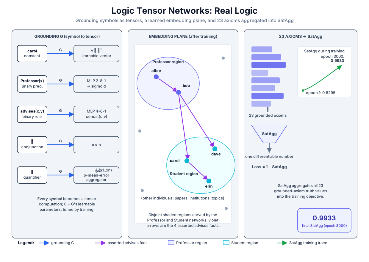The grounding maps every symbol to a tensor computation (left), the learned 2-D plane carves disjoint Professor and Student regions around the moving embeddings (center), and the 23 grounded axioms aggregate into the single differentiable number SatAgg that training pushes from 0.5295 to 0.9933 (right). Original diagram by the authors, created with AI assistance.

The connectives: the stable product configuration

With atoms grounded, compound formulas need connectives, and Part I built the menu. Real Logic's reference formulation recommends one specific selection, the stable product configuration [1], and the systematic operator analysis of differentiable fuzzy logics explains why it wins: its gradients are nonzero for both arguments everywhere in the interior of the unit square, which is where the sigmoids and the clamps keep every truth value, in contrast to the Gödel operators, which route the whole gradient to one argument, and the Łukasiewicz pair, whose clipping creates a zero-gradient dead zone [3]. Here are the four choices, together with the partial derivatives gradient descent actually consumes:

connective	operator	formula	$\partial/\partial a$	$\partial/\partial b$
$a \wedge b$	product t-norm $T_P$	$a \cdot b$	$b$	$a$
$a \vee b$	probabilistic sum $S_P$	$a + b - ab$	$1 - b$	$1 - a$
$\neg a$	standard negation $N_S$	$1 - a$	$-1$	—
$a \rightarrow b$	Reichenbach implication $I_R$	$1 - a + ab$	$b - 1$	$a$

Each row is a reasoned choice, not a default. The product t-norm was the fuzzy-to-neural chapter's dense-gradient winner: unlike the Gödel minimum, which routes the entire gradient to the single weakest conjunct and starves the rest, the product's leave-one-out partials $\partial(ab)/\partial a = b$ keep every conjunct learning. The probabilistic sum is its De Morgan dual under $N_S$: the closed form s_probsum of tnorms.py (lines 128–130), which that module checks against the dual construction $1 - T_P(1-a, 1-b)$ with deviation exactly zero. The Reichenbach implication is not the Goguen residuum of the product (that arrow contains the quotient $b/a$, consequent over antecedent, whose gradient is singular as the antecedent $a \to 0$); it is the material arrow built from the stable pair, and that identity is worth one line of algebra. Define it as $\neg a \vee b$ under the configuration's own negation and disjunction:

$$I_R(a, b) \;=\; S_P\big(N_S(a),\, b\big) \;=\; (1 - a) + b - (1 - a)\,b \;=\; 1 - a + b - b + ab \;=\; 1 - a + ab .$$

The middle step expands $S_P(x, b) = x + b - xb$ at $x = 1 - a$; the $+b$ and $-b$ cancel, leaving a polynomial that is smooth everywhere, with no case split, no quotient, and no kink. The companion does not take the identity on faith: ltn.py lines 507–511 assert $I_R(a,b) = S_P(1-a, b)$ with deviation exactly $0.0$ on the dyadic grid of tnorms.py, where every value is an exact binary float. The partials carry the semantics of learning through an implication: $\partial I_R/\partial b = a$ says the gradient flowing into the consequent is gated by the truth of the antecedent (a fuzzy shadow of modus ponens: the rule only teaches its head where its body holds), and $\partial I_R/\partial a = b - 1 \le 0$ says raising the antecedent can only lower the implication, unless the consequent is already fully true. The implementation is two lines (ltn.py lines 120–125):

def implies(a, b):
    # Reichenbach implication  I_R(a, b) = 1 - a + a·b.
    ...
    return 1.0 - a + a * b

One more ingredient comes from Part I with its price tag attached. The word stable refers to two clamping projections, $\pi_0(a) = (1-\varepsilon)a + \varepsilon$ and $\pi_1(a) = (1-\varepsilon)a$, which bound truth values away from exactly 0 and exactly 1 before they enter any operation that is singular there [1]; the paper leaves $\varepsilon$ unspecified beyond being small, and the companion (following the reference implementation's default) sets $\varepsilon = 10^{-4}$. The fuzzy-to-neural chapter committed the exhibit rather than the argument: in fuzzy_grad.py (lines 310–343), a single exactly-false grounding turns the log-product loss into a literal inf with an infinite gradient, while the clamped version is bounded by $-\log \varepsilon \approx 9.21$ per term and gradient magnitude $(1-\varepsilon)/\varepsilon \approx 10^4$. This chapter imports $\pi_0$, $\pi_1$, and $\varepsilon$ from that module (ltn.py line 79) and applies them in exactly one place: inside the quantifier aggregators, where the next section shows the same explosion waiting.

Quantifiers as generalized means

Here is the construction that separates Real Logic from everything in Part II. A quantified formula $\forall x\, \phi(x)$ is grounded by evaluating $\phi$ on every individual, producing a vector of instance truths $a_1, \ldots, a_n$, where $n$ is the number of grounded instances (here $n = 13$ for one variable ranging over the individuals, and $n = 169$ for two). The quantifier is then an aggregator: a differentiable function collapsing those $n$ numbers into one. Real Logic uses the family of generalized means with exponent $p$, a real number at least 1 that acts as an outlier-sensitivity dial [1]. The existential quantifier ∃ is the $p$-mean (read the display as: raise each instance truth $a_i$ to the power $p$, average the results, the summation sign $\sum_{i=1}^{n}$ adding the $n$ powered truths one instance $i$ at a time, and take the $p$-th root),

$$A_{pM}(a_1, \ldots, a_n) \;=\; \left( \frac{1}{n} \sum_{i=1}^{n} a_i^{\,p} \right)^{1/p},$$

and the universal quantifier ∀ is the $p$-mean-error, which averages the deviations from truth $1 - a_i$ and subtracts the result from 1:

$$A_{pME}(a_1, \ldots, a_n) \;=\; 1 - \left( \frac{1}{n} \sum_{i=1}^{n} (1 - a_i)^{\,p} \right)^{1/p}.$$

Read the dial before the derivation. At $p = 1$ both reduce to the plain arithmetic mean: every instance counts equally, and a universal can score 0.9 while one instance sits at 0. As $p$ grows, the power sum is dominated by its largest terms: the largest $a_i$ for $A_{pM}$ (the optimist, leaning on the best witness), the largest error $1 - a_i$ for $A_{pME}$ (the pessimist, leaning on the worst violation). In the limit the means become the Gödel quantifiers. To see it for $A_{pME}$, write $e_i = 1 - a_i$ for the errors and $e_{\max} = \max_i e_i$, and squeeze the inner term:

$$\left(\tfrac{1}{n}\right)^{1/p} e_{\max} \;=\; \left( \frac{1}{n}\, e_{\max}^{\,p} \right)^{1/p} \;\le\; \left( \frac{1}{n} \sum_i e_i^{\,p} \right)^{1/p} \;\le\; \left( \frac{1}{n} \cdot n\, e_{\max}^{\,p} \right)^{1/p} \;=\; e_{\max}.$$

The lower bound keeps only the largest term of the sum; the upper bound replaces every term by it. Since $(1/n)^{1/p} \to 1$ as $p \to \infty$ (the $p$-th root of a fixed fraction tends to 1), both bounds converge to $e_{\max}$, so $A_{pME} \to 1 - \max_i (1 - a_i) = \min_i a_i$: the worst instance alone decides, which is exactly the Gödel "for all" and exactly the sparse gradient the fuzzy-to-neural chapter warned against. The companion fixes $p = 2$ (ltn.py line 101), a stated compromise: already tilted toward the falsest instances, not yet starving the rest.

Now the chapter's main derivation: the gradient of $A_{pME}$ with respect to one instance truth $a_i$, every step shown. Name the inner power mean $M$, so the computation is a three-link chain:

$$e_i = 1 - a_i, \qquad M = \frac{1}{n} \sum_{j=1}^{n} e_j^{\,p}, \qquad A_{pME} = 1 - M^{1/p}.$$

Link one, the aggregate through the power mean. Differentiating $1 - M^{1/p}$ with respect to $M$ by the power rule:

$$\frac{\partial A_{pME}}{\partial M} \;=\; -\,\frac{1}{p}\, M^{\frac{1}{p} - 1}.$$

Link two, the power mean through the error. Only the $j = i$ term of the sum depends on $e_i$, and differentiating $e_i^{\,p}$ gives $p\, e_i^{\,p-1}$:

$$\frac{\partial M}{\partial e_i} \;=\; \frac{1}{n} \cdot p\, e_i^{\,p-1}.$$

Link three, the error through the instance. From $e_i = 1 - a_i$, simply $\partial e_i / \partial a_i = -1$. Multiplying the three links, the $p$ from link two cancels the $1/p$ from link one, and the two minus signs cancel each other:

$$\frac{\partial A_{pME}}{\partial a_i} \;=\; \left(-\frac{1}{p} M^{\frac{1}{p}-1}\right) \cdot \left(\frac{p}{n}\, e_i^{\,p-1}\right) \cdot (-1) \;=\; \frac{1}{n}\; e_i^{\,p-1}\; M^{\frac{1-p}{p}}.$$

Read the two factors that survive. The factor $e_i^{\,p-1}$ is per-instance: each instance receives gradient in proportion to the $(p-1)$-th power of its own violation. At $p = 2$ this is simply $e_i / (n \sqrt{M})$, gradient proportional to how false the instance currently is; the ratio of gradients between two instances is $(e_i / e_j)^{p-1}$, so as $p$ grows the aggregator concentrates its entire learning signal on the most-violated instances. The semantics of "for all" becomes a curriculum: the optimizer is always working hardest on the worst counterexamples to the axiom, and the dial $p$ sets how single-minded that focus is [1]. The factor $M^{(1-p)/p}$ is global, and it is the trap: as an axiom approaches full satisfaction every $e_j \to 0$, so $M \to 0$, and $M^{(1-p)/p}$ (which is $M^{-1/2}$ at $p = 2$) diverges. This is the quantifier-level version of the log explosion, and it is why the stable variants clamp their inputs with $\pi_1$ before the power mean: with $e_i = 1 - (1-\varepsilon) a_i \ge \varepsilon$, the mean obeys $M \ge \varepsilon^p$, so the exploding factor is bounded by $\varepsilon^{1-p}$ and the chain picks up one extra $(1-\varepsilon)$ from $\partial e_i/\partial a_i = -(1-\varepsilon)$. The implementation is the derivation, line for line (ltn.py lines 141–149):

def agg_forall(a: np.ndarray, p: int = P) -> tuple[float, np.ndarray]:
    """Stable A'_pME and its gradient ∂A/∂a_i (derivation above)."""
    n = a.size
    e = 1.0 - pi_1(a)                       # e_i = 1 - (1-ε)a_i  ∈ [ε, 1]
    m = float(np.mean(e ** p))              # M = (1/n) Σ e_i^p  ≥ ε^p
    val = 1.0 - m ** (1.0 / p)              # A_pME = 1 - M^{1/p}
    # ∂A/∂a_i = (1-ε)/n · e_i^{p-1} · M^{(1-p)/p}
    grad = (1.0 - EPS) / n * e ** (p - 1) * m ** ((1.0 - p) / p)
    return val, grad

The existential mirror agg_exists (ltn.py lines 160–168) runs the same chain on $b_i = \pi_0(a_i)$ without the final flip, giving $\partial A_{pM}/\partial a_i = \frac{1-\varepsilon}{n} b_i^{\,p-1} M^{(1-p)/p}$: the gradient leans on the truest witnesses, the instances already closest to satisfying the existential.

The knowledge base as one differentiable number

A Real Logic theory is a set of closed formulas, and its training objective is their aggregated truth, SatAgg. The companion grounds the real Volume 2 axioms, not a toy imitation: the 14-axiom TBox (terminological box, the schema-level axioms) lives in ontology.py lines 125–174, and ltn.py translates into first-order form every axiom that mentions only the model's grounded signature of seven concepts and the advises role; the grandAdvisor role chain, the Dean, TenuredStudent, and TenuredStudentAdvisor axioms, and the two authored-role axioms fall outside that signature and are not grounded. The committed run prints the inventory:

[1] the grounded theory: 23 axioms from Volume 2's ontology.py, 306 parameters
    abox      13 axiom(s)   ABox typings C(a)
    disjoint   1 axiom(s)   ∀x ¬(Prof(x) ∧ Stud(x))          [TBox 6]
    subsume    3 axiom(s)   the ladder ∀x C(x) → D(x)        [TBox 1-3]
    dom/rng    2 axiom(s)   adv domain ∀ + range-∃           [TBox 5, 4]
    facts      4 axiom(s)   asserted advises(a, b) atoms

The 13 typings from the ABox (assertional box, the ontology's ground facts) and the 4 advises facts are ground atoms, so their truth is a single predicate evaluation. The disjointness Professor ⊓ Student ⊑ ⊥ (Volume 2's description-logic notation: read ⊑ as "is subsumed by", ⊓ as concept intersection, ⊤ as the concept containing everything, and ⊥ as the empty concept; ontology.py line 143) becomes $\forall x\, \neg(\mathrm{Prof}(x) \wedge \mathrm{Stud}(x))$: instance truths $u_x = 1 - \mathrm{Prof}(x) \cdot \mathrm{Stud}(x)$, aggregated by $A_{pME}$ (ltn.py lines 325–334). The subsumption ladder Professor ⊑ Researcher, Student ⊑ Researcher, Researcher ⊑ Person becomes three universally quantified Reichenbach implications. The advises domain axiom ∃advises.⊤ ⊑ Researcher (ontology.py line 138) becomes $\forall x \forall y\, \mathrm{advises}(x,y) \rightarrow \mathrm{Res}(x)$, a $13 \times 13$ instance grid. And the one axiom that exercises ∃, Professor ⊑ ∃advises.Student (ontology.py line 133), nests the quantifiers:

$$\forall x \Big[ \mathrm{Prof}(x) \rightarrow \exists y \big( \mathrm{advises}(x, y) \wedge \mathrm{Stud}(y) \big) \Big],$$

computed inside-out exactly as the semantics composes (ltn.py lines 359–379): the inner conjunction fills a $13 \times 13$ grid $\mathrm{inner}_{xy} = \mathrm{ADV}_{xy} \cdot \mathrm{Stud}_y$, each row aggregates through $A_{pM}$ into an existence score $\mathrm{ex}_x$, each $u_x = I_R(\mathrm{Prof}_x, \mathrm{ex}_x)$ applies the arrow, and $A_{pME}$ closes the universal. Every operator in that pipeline is one from the two sections above, so the hand-written backward pass is nothing but their partials chained in reverse order.

SatAgg itself is a choice with a gradient, not an afterthought. The companion follows the framework's practical recommendation and reuses $A_{pME}$, at the same $p = 2$, over the 23 per-axiom truths $\mathrm{sat}_1, \ldots, \mathrm{sat}_{23}$ [1], and minimizes

$$L \;=\; 1 - \mathrm{SatAgg} \;=\; 1 - A_{pME}(\mathrm{sat}_1, \ldots, \mathrm{sat}_{23}), \qquad \frac{\partial L}{\partial\, \mathrm{sat}_k} \;=\; -\,\frac{1-\varepsilon}{23}\, (1 - (1{-}\varepsilon)\mathrm{sat}_k)^{\,p-1}\, M^{\frac{1-p}{p}} \;\le\; 0,$$

by the identical derivation, with the sign flipped by the outer $1 - {}$. Two consequences follow immediately. The gradient is never positive: raising any axiom's truth always lowers the loss. And the most violated axiom gets the largest push, because the per-axiom factor is again the violation to the power $p - 1$; SatAgg runs the same worst-first curriculum across axioms that each universal runs across instances. The forward-plus-backward pass is ltn.py lines 388–396, and the training loop is plain full-batch gradient descent, $\theta \leftarrow \theta - \eta\, \partial L/\partial \theta$, where the parameter vector $\theta$ collects all 306 learnable numbers and the learning rate $\eta = 2.0$ scales each step, run for 3000 epochs (ltn.py lines 443–447). Before any of it runs, the module certifies the entire hand assembly: the maximum gap between the analytic gradient and a central finite difference, over all 306 parameters, is $1.092 \times 10^{-10}$ (output block [3]), which is the numerical signature of a correctly chained derivation. The committed trace:

[4] training: full-batch GD on L = 1 − SatAgg  (η = 2.0, 3000 epochs)
    epoch :  SatAgg    1 − SatAgg
        1 :  0.5295    0.4705
       10 :  0.7425    0.2575
      100 :  0.9564    0.0436
      500 :  0.9890    0.0110
     1000 :  0.9931    0.0069
     2000 :  0.9933    0.0067
     3000 :  0.9933    0.0067

The per-group satisfactions, before and after, are where the theory meets this particular world. Read the committed table row by row:

group	axioms	before	after	what the row says
abox	13	0.4670	0.9991	randomly initialized MLPs answer near 0.5 on everything; the typings are the easiest axioms, pure supervised attraction toward 1
disjoint	1	0.7301	0.9986	high before training by ignorance: two predicates near 0.5 give a conjunction near 0.25 and a negation near 0.75; the real work comes later
subsume	3	0.7545	0.9987	implications with a near-0.5 antecedent start near $1 - 0.5 + 0.25 = 0.75$; training must keep them true while the ABox drives the antecedents to 1
dom/rng	2	0.6669	0.9776	the hardest group, and the lowest finisher: the nested ∃ axiom must coordinate three predicates across 169 pairs at once
facts	4	0.5200	0.9995	four ground atoms pulled to 1, the binary analogue of the ABox row

The disjointness row deserves the closer look, because it is the one axiom that supplies negative pressure. Every other axiom is satisfied by the all-true assignment: a lazy optimizer could satisfy all of them at once by driving every predicate toward 1 on every individual. Disjointness alone punishes that: as the ABox pushes Stud(carol) toward 1, the instance truth $1 - \mathrm{Prof}(\mathrm{carol}) \cdot \mathrm{Stud}(\mathrm{carol})$ can stay high only if Prof(carol) is pushed toward 0. Its gradient $\partial u_x / \partial \mathrm{Prof}_x = -\mathrm{Stud}_x$ presses a predicate downward, and unlike the implications' negative antecedent pressure (their $b - 1$ partials, which vanish once the consequents saturate at 1), this pressure persists at saturation: disjointness is the only axiom whose satisfaction requires driving a predicate toward 0, and it is what carves the Professor and Student regions apart in the learned plane rather than letting them dissolve into one blob of universal truth.

The probes that keep it honest

A satisfaction score of 0.9933 says the training worked; it does not say the model learned logic rather than a lookup table. So the committed run interrogates the trained grounding with queries that were never per-axiom training targets (plus a per-atom re-check of the four trained facts), and asserts every verdict (ltn.py lines 540–557):

[6] the learned world — truth values for the five people
    (Researcher and Person are NEVER asserted: the subsumption
    ladder alone entails them — gradient descent as inference)
    individual   Prof    Stud    Researcher  Person
    alice       0.9991  0.0014  0.9988      0.9979
    bob         0.9990  0.0014  0.9985      0.9976
    carol       0.0008  0.9999  0.9990      0.9987
    dave        0.0004  0.9999  0.9983      0.9980
    erin        0.0005  0.9999  0.9986      0.9984
    entailed minima over the five: Researcher ≥ 0.9983, Person ≥ 0.9976

    held-out probes:
    Professor(carol) = 0.0008   (< 0.3 asserted; carol is typed Student)
    max_x Prof(x)·Stud(x) = 0.0018 at x = p3   (< 0.25 asserted: disjointness holds everywhere)
    the 4 asserted advises facts:
      advises(alice,bob)     0.9995
      advises(bob,carol)     0.9999
      advises(bob,dave)      0.9998
      advises(carol,erin)    0.9993

Three readings. First, the Researcher and Person columns are emergent entailment: no ABox axiom ever asserts Researcher(alice) or Person(carol), yet all five people end at or above 0.9976 in both, because the only way to satisfy the ladder implications while the ABox holds their antecedents at 1 is to make the consequents true. Gradient descent has performed, numerically, the inference Volume 2's completion algorithm performed symbolically. Second, Professor(carol) lands at 0.0008, not at the 0.5 of ignorance: nothing asserted it false, but the disjointness axiom transmitted Stud(carol) = 0.9999 into downward pressure on Prof(carol). Third, the conjunction $\mathrm{Prof}(x) \cdot \mathrm{Stud}(x)$, the fuzzy rendering of the intersection Professor ⊓ Student (the concept whose asserted emptiness is what makes Volume 2's TenuredStudent provably unsatisfiable), peaks at 0.0018 over all 13 individuals, and the probe reads the trained values more strictly than training ever did: it replaces the disjointness axiom's trained $p$-mean over instances with a hard max. In the crisp ontology that intersection is exactly empty; the trained grounding leaves it nearly empty, which is both the success and the precise measure of the gap.

The last probe checks the claim on which the whole fuzzy pillar leans: that Real Logic is a generalization of classical logic, not a replacement. On crisp inputs, values in $\lbrace 0, 1 \rbrace$, the stable product connectives are algebraically the Boolean ones: $a \cdot b$ is AND, $a + b - ab$ is OR, $1 - a$ is NOT, $1 - a + ab$ is the material conditional. The companion asserts every corner of all four truth tables with exact equality, no tolerance (ltn.py lines 467–472), and then evaluates one full quantified axiom on crisp indicator vectors (ltn.py lines 474–498). For $\forall x\, \mathrm{Stud}(x) \rightarrow \mathrm{Res}(x)$ with Researcher taken as its classical closure (the crisp indicator vector that is 1 exactly on the professors and students, the set the subsumption ladder entails), every instance is exactly 1, so the error mean is exactly 0 and the unclamped $A_{pME}$ returns exactly $1 - 0^{1/2} = 1.0$, the classical truth of a true universal (the clamps are a trainability device and are switched off here, since $\pi_1$ would shift a crisp 1 to $1 - \varepsilon$). The classically false axiom $\forall x\, \mathrm{Prof}(x) \rightarrow \mathrm{Stud}(x)$ is the more instructive trace, and the printed 0.6078 can be reproduced by hand. The instance vector has $I_R(1, 0) = 1 - 1 + 0 = 0$ at the two professors, alice and bob, and $I_R(0, \cdot) = 1$ at the other eleven individuals, so across the thirteen individuals the error vector holds two 1s and eleven 0s:

$$M \;=\; \frac{2}{13} \approx 0.1538, \qquad A_{pME} \;=\; 1 - M^{1/2} \;=\; 1 - 0.3922 \;=\; 0.6078 .$$

The verdict survives the fuzzification (true axioms sit at exactly 1, false axioms strictly below 1, and the violating instances themselves at exactly 0), but the value 0.6078 is graded, not the classical hard 0; recovering that would need $p \to \infty$, the Gödel limit derived above. This is the continuity claim between fuzzy and classical logic made checkable: not asserted in prose but held by assert statements in committed code.

Beyond satisfaction: what a trained grounding is for

Maximizing SatAgg is learning, but the trained grounding supports more than its own training objective [1]. Querying is immediate: any closed formula of the language, including ones never seen during training, evaluates to a truth degree under the final parameters; the held-out probes above are exactly this. Reasoning by refutation inverts the machinery: to ask whether the theory entails $\phi$, add $\neg\phi$ and try to maximize satisfaction; if no parameter setting keeps the augmented theory satisfiable to a high degree, the failed search is evidence for entailment, and if the search instead succeeds, the grounding it finds satisfies the theory while falsifying $\phi$, and is itself the counterexample that refutes entailment. And the framework's early flagship application is semantic image interpretation, where individuals are grounded not as learnable embeddings but as the feature vectors of detected objects, so the axioms regularize a perception network's outputs toward logical coherence [4]; the design is ltn.py with the embedding matrix swapped for a vision model's outputs.

The honest cost is written in the shape of the computation. Grounding a formula enumerates instances: one quantified variable over $n$ individuals costs $n$ evaluations, and $k$ distinct quantified variables cost $n^k$, exponential in $k$. Our nested axiom already fills a $13 \times 13 = 169$ grid for $k = 2$; the same axiom over a knowledge graph with $10^5$ entities would demand $10^{10}$ pair evaluations per epoch. The framework names the escape hatches: diagonal quantification quantifies over paired tuples that walk one shared index instead of the full product grid, and guarded quantification restricts the instances to those satisfying a cheap symbolic condition before the neural evaluation runs, shrinking $n^k$ to the guard's support [1]. Both are domain restrictions a modeler must choose, not optimizations a compiler finds.

The unsolved part

The number the run ends on, SatAgg = 0.9933, is not a proof of anything, and the aggregation mathematics says precisely why. $A_{pME}$ at finite $p$ is an average, and averages absorb localized violations: over the 169-instance grid of a two-variable universal, a single instance at truth 0 among 168 perfect ones yields $M = 1/169$ and a satisfaction of $1 - \sqrt{1/169} = 1 - 1/13 \approx 0.923$. An axiom can read "92% satisfied" while being, classically, simply false, with a concrete counterexample sitting in the grid. Volume 2's reasoner could never do this; its entailments were all-or-nothing and came with derivations. Second, truth degrees are not calibrated probabilities. The 0.9995 the trained model assigns to advises(alice, bob) is not a 99.95% chance of anything: it is a sigmoid output shaped by loss pressure, and the fuzzy-logic tradition itself is explicit that degrees of truth and degrees of belief are different quantities with different laws [5]. Part II's numbers were probabilities in the exact, model-counting sense; Real Logic's numbers are positions on a satisfaction dial, and thresholding or comparing them across predicates has no semantic license. Third, nothing prevents satisfaction by geometric accident: the objective constrains 306 parameters through 23 axioms evaluated at 13 points, and the MLPs are free to carve the plane in any way that scores well there, including ways that would violate the axioms badly at embeddings just off the trained ones. The held-out probes were chosen because they could have failed; passing them is evidence, not certification. Whether satisfaction maximization can be given certificates (bounds on hidden violations, calibration of its degrees, guarantees off the training grid) is open, and the field's working answer for applications that need guarantees is to change pillars back: keep the exactness of Part II's circuits and attack their cost instead, which is exactly where the next chapter goes.

Why it matters

This chapter completes the volume's second pillar. DeepProbLog showed the probabilistic route to trainable logic: exact semantics, propositional core, gradients through model counting. Logic Tensor Networks shows the fuzzy route: quantified first-order syntax kept intact, exactness surrendered, gradients through generalized means. Every integration system in the rest of this volume sits somewhere on the axis these two ends define, and the trade is now quantified rather than rhetorical: a 0.9933 aggregate with worst-first gradient scheduling here, exact query probabilities at compilation cost there. The failure modes documented here are also load-bearing for Volume 5: uncalibrated confidence and averaged-away violations are precisely the trust problems its faithfulness and calibration chapters probe, and the worst-instance curriculum inside $A_{pME}$ foreshadows the verifier-guided training loops at the frontier.

Key terms

• Real Logic: the fully differentiable first-order language of Logic Tensor Networks; first-order syntax, semantics in $[0,1]$, every operator chosen to carry gradients.
• Grounding $\mathcal{G}$: the mapping from symbols to tensors; constants to learnable vectors, predicates to differentiable functions into $[0,1]$, formulas to compositions of both.
• Stable product configuration: the recommended operator menu; product t-norm, probabilistic sum, standard negation, Reichenbach implication $1 - a + ab$, plus the clamps $\pi_0, \pi_1$ at the aggregators.
• Generalized $p$-mean ($A_{pM}$, $A_{pME}$): the quantifier aggregators; $p$ dials outlier sensitivity, $p \to \infty$ recovers max (for $A_{pM}$) and min (for $A_{pME}$), and the gradient $\frac{1}{n} e_i^{p-1} M^{(1-p)/p}$ concentrates on the most-violated instances.
• SatAgg: the aggregated truth of the whole theory, here $A_{pME}$ over the per-axiom truths; the training loss is $1 - \mathrm{SatAgg}$.
• Negative pressure: the force a negated axiom (here disjointness) exerts to push truth values down, without which satisfaction maximization degenerates to "everything is true."
• Crisp recovery: the collapse of Real Logic to classical logic on $\lbrace 0,1 \rbrace$ inputs, asserted exactly in the companion.
• Diagonal / guarded quantification: the escape hatches from the $n^k$ grounding cost of $k$ quantified variables; shared-index tuples, or symbolic pre-filters on the instance grid.

Where this leads

Real Logic bought first-order syntax by giving up guarantees; Part II's circuits held the guarantees but paid for them in compilation and in CPU-bound, pointer-chasing evaluation. The frontier's answer to that cost is not a new semantics but new hardware discipline: flatten the compiled circuits into dense tensor layers, batch millions of world-weight products onto the same accelerators that train the neural predicates, and make exact inference fast enough to sit inside a training loop at scale. That is the subject of the next chapter, GPU-Native NeSy, where the two pillars stop competing for elegance and start competing for throughput.

---

Companion code: examples/integration/ltn.py grounds Volume 2's axioms into the 306-parameter Real Logic model, derives every gradient by hand (certified against central finite differences to $1.092 \times 10^{-10}$), trains SatAgg from 0.5295 to 0.9933, and asserts every probe quoted in this chapter. It imports its conjunction and disjunction from tnorms.py (negation and the Reichenbach arrow are local two-liners asserted against that module's dyadic grid), its clamps from fuzzy_grad.py, and its axioms from examples/symbolic/ontology.py. Run python3 examples/integration/ltn.py to reproduce every number; two runs print byte-identical output.