GPU-Native NeSy: KLay and Lobster

📍 Where we are: Part III · Differentiable Frameworks — Chapter 11. Logic Tensor Networks rebuilt first-order logic as operations on tensors so that axioms could become a loss; this chapter keeps the semantics exact and rebuilds the machinery instead: the same inference Part II certified, re-laid-out as matrix products and layered array passes that ride the same hardware as the neural half.

Every exact system in this volume so far has carried a quiet asterisk: it runs on the wrong hardware. The distribution semantics, weighted model counting, compiled circuits, the gradient semiring, all were built as recursive programs chasing pointers through irregular data structures on a CPU (central processing unit), while the neural networks they integrate with scream through batched dense linear algebra on GPUs (graphics processing units, the accelerators deep learning runs on). This chapter closes that gap without touching the semantics. The claim to be tested is architectural: exactness is not what made neuro-symbolic (NeSy, the abbreviation in this chapter's title) systems slow; the memory layout was. Two tensorizations make the case runnable on our academic world, one turning relations into matrices so that a rule application is a matrix product, one turning a compiled circuit into layers so that evaluation is a sequence of vectorized gathers and reductions. A third system, treated at the language level, lowers a whole Datalog engine onto the GPU.

The simple version

Imagine a warehouse that fulfills orders one at a time. A single picker takes an order slip, walks to a shelf, reads a note taped there pointing to another shelf, walks there, and so on until the order is assembled: correct, but mostly walking. Now reorganize the same warehouse into staging rows: everything needed at step one sits in row one, everything needed at step two in row two, and a whole cart of a thousand order slips rolls down the rows together, each row serviced in one sweep. Not a single item changed, not a single order is filled differently; only the floor plan changed, and the walking disappeared. That is this chapter. The "orders" are exact logical queries, the "notes pointing to other shelves" are the recursive evaluators of Part II, and the reorganized floor plan is what TensorLog does to rules and KLay does to circuits.

What this chapter covers

• The bottleneck named precisely: Part II's pipeline (ground, compile, evaluate) is exact, but its evaluators are interpreted, pointer-chasing node-by-node walks with irregular memory access, while the neural half enjoys batched dense kernels; the systems question is whether exact logic can ride the same hardware.
• Logic as linear algebra: each of the 5 relations becomes a 13-by-13 Boolean adjacency matrix, a body atom a matrix-vector product, and grandAdvisor = advises ∘ advises (∘ is relation composition: follow one advises edge, then another) one matrix product whose support the companion proves equal, as a set, to Volume 1's forward-chained facts.
• What the matrix view buys and hides: batched k-hop reachability and differentiability for free; hidden underneath, matrix entries are proof-path counts, not truth values, so Boolean semantics needs an explicit clamp, worked on the fact with two derivations.
• KLay's three algorithms on our own circuit: layerization by node height, tensorization into flat integer buffers, and evaluation by gather plus segment-reduce, matching the recursive weighted model count to 1e-10 over 1000 weight vectors.
• The log semiring done right: why long products underflow, the logsumexp max trick derived with its residual bounded, and the committed linear-versus-log agreement at 1e-9.
• An honest benchmark and the language level: a measured timing table framed as what it is (a NumPy proxy for the GPU story), Lobster's lowering of Scallop's Datalog onto the GPU, and a map of which system owns which layer of the emerging stack.

The bottleneck, named precisely

Recall what Part II actually built. Circuits gave us the pipeline ground, compile, evaluate: ground the probabilistic program into a propositional formula, compile it once into a smooth deterministic decomposable circuit, then answer every query by one bottom-up pass, linear in circuit size, one semiring operation (one generalized add, written ⊕, or one generalized multiply, written ⊗) per edge. The trouble is the word pass. The evaluator in circuit.py (lines 336–366) walks a topologically sorted list of heterogeneous node tuples, follows child indices scattered through memory, and dispatches on node kind at every step: a pointer dereference, a branch, and a little arithmetic per visit, exactly the access pattern that starves a modern processor, whose speed comes from predictable, contiguous, wide reads. Meanwhile the neural half spends its time in matrix multiplications: dense, regular, batched, served by hardware built for nothing else. Trained jointly, as in DeepProbLog, the profile is lopsided: the perception network finishes its batch in milliseconds of accelerator time, then waits while interpreted Python evaluates circuits one query at a time (the evaluator is recursively defined but executes as that loop over the topological order; the module's output labels it "recursive", and this chapter keeps the label when quoting). The cost concentrates exactly there: compilation is paid once, but training re-evaluates the compiled circuit at every gradient step, and this recurring circuit evaluation has been identified as one of the major bottlenecks of current neuro-symbolic architectures [1].

So the systems question of this chapter: can exact inference, with its semantics untouched, be re-expressed in the vocabulary the hardware speaks, which is to say batched dense array operations? Two published answers say yes, at two different levels of the stack. TensorLog answers at the level of rules: encode relations as adjacency matrices and a Datalog rule application becomes a matrix product, differentiable for free [2]. KLay answers at the level of circuits: reorganize a compiled circuit into layers of independent nodes and evaluation becomes a short sequence of vectorized gathers and segmented reductions [1]. A third system, Lobster, answers at the level of the language, lowering the whole of Scallop's provenance-carrying Datalog onto the GPU [3]; we return to it once the first two answers have run. The companion module tensor_ops.py miniaturizes the first two on the academic world, in plain NumPy, with every semantic claim guarded by an assert; the only thing it cannot miniaturize is the silicon, and it says so.

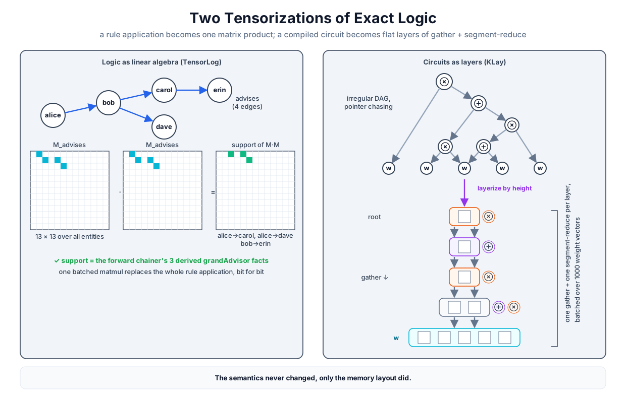The two tensorizations side by side: a rule application collapsed into one matrix product on the left, and the same compiled circuit from the circuits chapter reorganized into five flat layers evaluated by gather and segment-reduce on the right; neither move alters a single answer.

Original diagram by the authors, created with AI assistance.

Logic as linear algebra: relations become matrices

Start with notation. The academic knowledge graph from Volume 3's kg.py has 13 entities (ENTITIES, kg.py line 49: alice, bob, carol, cmu, dave, erin, logic, mit, ml, nesy, p1, p2, p3, in sorted order) and 5 base relations carrying 18 asserted edges. Write $N$ for the number of entities, so $N = 13$, and give every entity a fixed integer index through the dictionary E_ID (kg.py line 53). For each relation $r$, define its adjacency matrix $M_r$, an $N \times N$ array of zeros and ones with

$$M_r[h, t] \;=\; \begin{cases} 1 & \text{if the fact } (h, r, t) \text{ is asserted,} \\ 0 & \text{otherwise,} \end{cases}$$

where $h$ indexes the head (source) entity of the edge and $t$ the tail (target). The companion builds all five matrices directly from the triple store (tensor_ops.py lines 88–96):

def rel_matrix(rel: str) -> np.ndarray:
    """The 13x13 0/1 adjacency matrix of one relation over the FULL graph
    (kg.TRIPLES — forward chaining runs on the full fact base, so the
    matmul must too):  M_r[E_ID[h], E_ID[t]] = 1  iff  (h, r, t) holds."""
    m = np.zeros((N_E, N_E))
    for h, r, t in kg.TRIPLES:
        if r == rel:
            m[kg.E_ID[h], kg.E_ID[t]] = 1.0
    return m

An entity becomes a one-hot vector: a row of $N$ numbers, all zero except a single one at the entity's index. Write $v_{\text{alice}}$ for alice's one-hot row. Now watch what ordinary matrix algebra does to logic. The product of a row vector with a matrix is defined coordinate-wise as $(v M_r)[t] = \sum_{h} v[h]\, M_r[h, t]$, where the sum runs over all $N$ head indices. With $v = v_{\text{alice}}$, every term with $h \ne \text{alice}$ vanishes, leaving $(v_{\text{alice}} M_r)[t] = M_r[\text{alice}, t]$: the product simply reads off alice's row, a vector with a one at every entity alice is $r$-related to. In logical terms, multiplying by $M_r$ applies one body atom: it maps the set "alice" to the set "everything alice $r$-relates to". This is TensorLog's founding observation: unification against a database of facts, the inner loop of every Prolog engine, is a sparse matrix-vector product, and therefore a chain of body atoms is a chain of such products [2].

Now the running rule. Volume 1's kb.py defines grandAdvisor by the Horn clause grandAdvisor(X, Z) :- advises(X, Y), advises(Y, Z). Read the symbol :- as "if": the head on the left, grandAdvisor(X, Z), holds whenever both body atoms on the right, advises(X, Y) and advises(Y, Z), hold. Two body atoms, so two products, which associativity lets us collapse into one matrix-matrix product first. Unpack the definition of the product of $M_{\text{advises}}$ with itself, entry by entry:

$$\big(M_{\text{advises}}\, M_{\text{advises}}\big)[x, z] \;=\; \sum_{y=1}^{N} M_{\text{advises}}[x, y]\; M_{\text{advises}}[y, z].$$

Each summand is a product of two entries that are each 0 or 1, so the summand is 1 exactly when both edges exist, that is, when $y$ is a middle person with advises$(x, y)$ and advises$(y, z)$ both asserted. Summing over all $N$ choices of $y$ therefore counts the advising 2-paths from $x$ to $z$: the entry is the number of distinct derivations of grandAdvisor$(x, z)$, one per binding of the rule's middle variable. The graph has four advises edges: alice→bob, bob→carol, bob→dave, carol→erin. Trace alice's row through the two hops by hand. First hop: $v_{\text{alice}} M_{\text{advises}} = v_{\text{bob}}$, the one-hot row at bob, because bob is the only person alice advises. Second hop: $v_{\text{bob}} M_{\text{advises}} = v_{\text{carol}} + v_{\text{dave}}$, a vector with ones at carol and dave, bob's two advisees. So exactly two entries of the alice row of the squared matrix light up, carol and dave, each with the value 1 (one 2-path each). The same trace from bob lights up erin alone, via carol; from everyone else the row is zero. Three nonzero entries in total.

That is precisely what Volume 1's forward chainer derived, and the companion refuses to let the coincidence pass unchecked. It computes the product, reads back its support (the set of index pairs holding a nonzero, decoded to entity names by support, tensor_ops.py lines 99–102), and asserts set equality against the chainer's derived facts, then re-derives every entry against a definitional path-count oracle (tensor_ops.py lines 325–336):

    # [a1] ONE matmul applies grandAdvisor(X,Z) :- advises(X,Y), advises(Y,Z).
    g2 = mats["advises"] @ mats["advises"]
    fc_grand = {(a[1], a[2]) for a in derived if a[0] == "grandAdvisor"}
    # THE claim: the product's support IS the forward chainer's derivation.
    assert support(g2) == fc_grand, "matmul support != forward-chain facts"

The committed run prints the verdict, together with the batching bonus:

[2] one rule, one matmul: grandAdvisor(X,Z) :- advises(X,Y), advises(Y,Z)
      (M_advises @ M_advises)[x, z] = Σ_y M[x,y] M[y,z] = #advising 2-paths
      support of the product : [('alice', 'carol'), ('alice', 'dave'), ('bob', 'erin')]
      Volume 1 forward chain  : the SAME 3 grandAdvisor facts (asserted
      as exact set equality; every entry equals the 2-path count)   PASS
      batched: 13 stacked one-hot sources = I₁₃ @ M² in one product;
      the alice row answers (alice, grandAdvisor, ?) = ['carol', 'dave']

The batching line is the whole economic argument in one identity. One query is a one-hot row times the squared matrix; a thousand queries are a thousand stacked one-hot rows times the squared matrix, still one product. Stacking all 13 possible sources gives the identity matrix $I_{13}$ (ones on the diagonal, zeros everywhere else: the matrix that multiplies without changing anything), so $I_{13}\, M^2 = M^2$ and the squared matrix is the complete answer table for every grandAdvisor query at once (tensor_ops.py lines 339–342 assert this and read the alice row back). Batching, the thing GPUs exist for, costs the logic nothing: it is a stack of rows.

What the matrix view buys, and what it hides

Two purchases come with the view. The first is k-hop reasoning by repeated multiplication: if one product applies one body atom, then the $k$-th power $M^k$ counts paths of length exactly $k$, and a query that composes $k$ relation hops is $k$ chained products, batched over sources exactly as above. The companion runs the powers of $M_{\text{advises}}$ and checks the whole profile against the graph (tensor_ops.py lines 345–351):

[3] k-hop by repeated matmul: powers of M_advises
      k   #pairs with a k-hop advising path   support
      1      4                                alice→bob, bob→carol, bob→dave, carol→erin
      2      3                                alice→carol, alice→dave, bob→erin
      3      1                                alice→erin
      4      0                                (none: DAG depth 3)

The advising graph is a directed acyclic graph (DAG) of depth 3, so the fourth power is the zero matrix; the module asserts the size sequence 4, 3, 1, 0 and pins the single 3-hop pair to alice→erin. The second purchase is the one this Part exists for: differentiability for free. A matrix product is a polynomial in its entries, so if the entries stop being frozen 0/1 constants and become learned parameters, gradients flow through rule application with no new mathematics; and if the choice of which matrix to multiply is made soft, a weighted mixture over relations, gradient descent can learn the rule itself. That move is the subject of the next chapter, and TensorLog is its direct ancestor [2].

Now the hidden cost, which the module shows rather than buries. Matrix entries are proof-path counts, not truth values. For grandAdvisor the distinction was invisible because advising is a tree (every entry of the square was 0 or 1, asserted at tensor_ops.py line 336), but one more rule exposes it. Consider sharesAuthor(P, Q) :- authored(X, P), authored(X, Q): two papers share an author when some person X wrote both. The first atom runs backward (from paper to person), which transposition handles: the matrix is $M_{\text{authored}}^{\top} M_{\text{authored}}$, where the superscript $\top$ marks the transpose, the matrix flipped across its diagonal so that rows and columns swap roles. Its diagonal entry at paper p1 is 2: two bindings of X (alice and bob, the co-authors) each complete a derivation of the same fact sharesAuthor(p1, p1). Logically one fact; arithmetically two paths. Boolean semantics needs an answer to be derivable or not, so the module applies the explicit clamp $\min(\cdot, 1)$, where the dot is a placeholder marking the slot the matrix entry fills: applied entrywise, every entry is capped at 1. It then asserts that clamping changes values but not support (tensor_ops.py lines 354–367). TensorLog itself makes the other choice: it keeps the raw entry as an unnormalized proof-count score, a sum over derivations rather than a truth value, a feature for ranking and a bug for logic [2]. The same care recurs for recursive rules: a transitive closure is no fixed power but a least fixpoint, so the module iterates $R \leftarrow \min(R + R M, 1)$, where $R$ is the reachability accumulated so far (initialized to $M$), until nothing changes (boolean_closure, tensor_ops.py lines 105–120), the matrix rendering of Volume 1's chase. On the citation graph it converges in $k = 2$ rounds:

      closure rule: R ← min(R + R·M_cites, 1) reaches its fixpoint at k = 2,
      support [('p2', 'p1'), ('p3', 'p1'), ('p3', 'p2')]
      == forward-chain citesTransitively (asserted set equality)   PASS

This is the honest summary of the first tensorization: chains of relations become products, sources batch into stacked rows, gradients come free, and the price is eternal vigilance about the difference between counting derivations and asserting truth. If you want probabilities with exact semantics rather than path counts, you need the second tensorization.

Circuits as layers: KLay's three algorithms on our own circuit

The circuits chapter compiled the query grandAdvisor(alice, Z) into a smooth circuit in deterministic decomposable negation normal form (d-DNNF): 3 variables (the annotated facts advises(alice, bob), advises(bob, carol), advises(bob, dave), with probabilities 0.9, 0.9, 0.85), 10 nodes, 10 edges, and a weighted model count (WMC) of 0.8865 that matched brute-force enumeration to 1e-12. That circuit is an irregular sparse DAG, the very shape GPUs were said to be bad at. KLay's response is three algorithms, each of which the companion reproduces on this exact circuit [1]. What they reorganize is the semiring-parametric circuit evaluation of algebraic model counting, one semiring operation per edge (⊕, the semiring sum, at OR nodes; ⊗, the semiring product, at AND nodes) [4]; what they run on are the standard compiled targets, d-DNNFs and their canonical cousins the sentential decision diagrams (SDDs) [5].

Algorithm one: layerize. Assign every node $n$ a height $h_n$: 0 for a leaf, $1 + \max$ of its children's heights for a gate (tensor_ops.py lines 156–161), and group nodes by height into layers. The payoff is an independence guarantee, and it follows from the definition in one step: every edge runs from a child $c$ to a parent $p$ with $h_p \ge 1 + h_c \gt h_c$, so no edge connects two nodes of the same height, so no node in a layer reads its own layer. An entire layer can be evaluated simultaneously, given only the layers below. One wrinkle: an edge may skip levels (a height-0 leaf feeding a height-4 gate). There the layerizer inserts a chain of unary pass-through nodes, one per skipped layer, so that afterwards every edge connects strictly adjacent layers and evaluation is a clean bottom-to-top sweep (tensor_ops.py lines 180–189). A pass-through is bookkeeping, not semantics: a one-child ⊕ segment, and reducing a single element returns it unchanged. The accounting is asserted, not narrated: layerized nodes = circuit nodes + pass-throughs, and buffer edges = circuit edges + pass-throughs (tensor_ops.py lines 388–392).

Algorithm two: tensorize. A layer must become something a vector processor can consume: flat integer buffers, not node objects. For each layer $l$ the companion records a gather-index array $S_l$ (for every incoming edge, the position in layer $l-1$'s value vector that it reads), segment offsets (where each node's contiguous block of edges begins), and the operator split: all ⊕ nodes (OR gates and pass-throughs) reordered first, all ⊗ nodes (AND gates) after, so one vectorized sum-reduction and one product-reduction cover the whole layer (tensor_ops.py lines 201–236). For the running circuit the committed run prints the result's shape and layer mix:

[5] KLay-lite: layerize by height, insert pass-throughs, flatten to buffers
      circuit                     vars  nodes  edges | layers  +pass  buffer edges
      ...
      grandAdvisor(alice, Z)         3     10     10 |      5      5            15
      ...
      grandAdvisor(alice, Z) layer mix — L1: 1 OR, 1 AND, 2 pass; L2: 0 OR, 1 AND, 2 pass; L3: 1 OR, 0 AND, 1 pass; L4: 0 OR, 1 AND, 0 pass

Ten circuit nodes spread over heights 0 through 4, five layers counting the leaves; five pass-throughs are inserted (the leaf advises(alice, bob), consumed only by the root at height 4, is escorted up through three of them), and the buffers carry 15 edges, exactly 10 + 5. To make "flat integer buffers" concrete, here is layer 1 as the layerizer actually builds it, read off a run of the committed code. Layer 0 holds the five literal slots, in order: advises(alice, bob), advises(bob, carol), ¬advises(bob, carol), advises(bob, dave), ¬advises(bob, dave).

layer-1 node	kind	segment of $S_1$	reads layer-0 slots	computes
slot 0	⊕ (OR)	positions 0–1	3, 4	the circuits chapter's smoothing gate pt = advises(bob, dave) ∨ ¬advises(bob, dave) (a binary OR, distinct from this chapter's unary pass-throughs)
slot 1	⊕ (pass)	position 2	1	advises(bob, carol), carried up
slot 2	⊕ (pass)	position 3	0	advises(alice, bob), carried up
slot 3	⊗ (AND)	positions 4–5	2, 3	¬advises(bob, carol) ∧ advises(bob, dave)

So $S_1 = [3, 4, 1, 0, 2, 3]$: six integers, three ⊕ segments starting at offsets 0, 2, 3, and one ⊗ segment after the split at position 4. No pointers survive; the layer is two flat arrays and an offset list.

Algorithm three: evaluate. With the buffers in hand, one layer costs exactly two array primitives: a gather (fancy indexing pulls every edge's source value into a contiguous array) and a segment-reduce (each node folds its contiguous block of gathered values with its semiring operator). This is algebraic model counting's evaluation, unchanged in meaning, re-expressed in the two primitives every array framework ships [4]. The inner loop is short enough to quote whole (tensor_ops.py lines 258–269, inside eval_batch):

        n = np.where(self.leaf_sign, w[:, self.leaf_var],
                     1.0 - w[:, self.leaf_var])
        for lay in self.layers:
            e = n[:, lay["S"]]                                    # gather
            out = np.empty((w.shape[0], lay["n_nodes"]))
            if lay["n_sum"]:
                out[:, :lay["n_sum"]] = np.add.reduceat(
                    e[:, :lay["split"]], lay["off_sum"], axis=1)
            if lay["n_sum"] < lay["n_nodes"]:
                out[:, lay["n_sum"]:] = np.multiply.reduceat(
                    e[:, lay["split"]:], lay["off_prod"], axis=1)
            n = out

Read the batching in the first line: w is a $B \times n_{\text{vars}}$ array, one row per weight vector in the batch (the batch size $B$ is 1000 here) and one column per circuit variable, and the leaf line materializes all $B$ leaf layers at once, taking $w$ for positive literals and $1 - w$ for negative ones. Every subsequent gather and reduce carries the batch dimension along untouched: the thousand circuit evaluations differ only in data, never in control flow, which is the definition of hardware-friendly. The unit of data moved is one gathered value per edge per row, and here the counts differ: the recursive evaluator reads one value per circuit edge, while the layered pass gathers one per buffer edge, which is the circuit's edges plus one edge per pass-through (15 versus 10 here; 1032 versus 238 on the deepest chain of the [5] table). The layered pass therefore moves strictly more data through memory. (Semiring applications, if anything, drop: reduceat folds a segment of $k$ gathered values with $k - 1$ applications, where $k$ is the segment's edge count, while the recursive evaluator folds each node from the semiring identity and spends $k$.) What changes decisively is the schedule: thousands of interpreted node visits become two vectorized primitives per layer. And the answers must not move at all. The module evaluates every circuit in the suite both ways, recursive and layered, and asserts agreement below $10^{-10}$ (tensor_ops.py lines 393–396):

[6] correctness: layered gather/reduce pass == recursive bottom-up pass
      circuit                     layered WMC      recursive WMC    |diff|
      ...
      grandAdvisor(alice, Z)      0.886500000000   0.886500000000   0.0e+00
      ...
      chain n=20                  0.999728026391   0.999728026391   0.0e+00

On every circuit, including the #P-wall chain family (the counting-hardness benchmark) from the weighted model counting chapter, whose label chain n=20 reads as a chain circuit over $n = 20$ variables (the coins, two per independent 2-coin chain), the difference is not merely under the tolerance; both passes execute the same additions and multiplications in a compatible order and agree bit for bit.

The log semiring, done right

Real deployments do not evaluate circuits on probabilities but on log-probabilities, for a concrete reason. A ⊗ node multiplies its children, and a deep circuit multiplies many probabilities: the product of $k$ factors of $\tfrac{1}{2}$ is $2^{-k}$, and double-precision floating point cannot represent any positive number below roughly $4.9 \times 10^{-324}$, so at $k = 1075$ the product silently flushes to exact zero and every gradient through it dies. The remedy is to carry $x = \log p$ (the natural logarithm, base $e$, the inverse of the exponential function $e^x$) instead of $p$ and translate the two semiring operations. The product translates itself: $\log(ab) = \log a + \log b$, so ⊗ becomes ordinary addition of log-values, which is why the log-space evaluator runs np.add.reduceat over its AND segments. The sum is the delicate one. A ⊕ node needs $\log(\sum_i p_i)$ from the children's log-values $x_i = \log p_i$, that is,

$$\bigoplus(x_1, \ldots, x_k) \;=\; \log \sum_{i=1}^{k} e^{x_i},$$

the logsumexp function, where $k$ is the number of children in the segment. Computing it literally would exponentiate first, re-creating the underflow it was meant to avoid (and overflow, if the $x_i$ were large). The max trick fixes both, and its derivation is three lines. Let $m = \max_i x_i$, the largest of the log-values. Factor $e^m$ out of every term of the sum, using $e^{x_i} = e^{m} e^{x_i - m}$:

$$\log \sum_{i=1}^{k} e^{x_i} \;=\; \log \Big( e^{m} \sum_{i=1}^{k} e^{x_i - m} \Big) \;=\; m + \log \sum_{i=1}^{k} e^{x_i - m},$$

the last step because the logarithm of a product is the sum of the logarithms. Now bound the residual sum $S = \sum_i e^{x_i - m}$. Every exponent satisfies $x_i - m \le 0$, so every term is at most $e^{0} = 1$; and the maximizing child contributes exactly $e^{m - m} = 1$. Hence $1 \le S \le k$, so the correction term $\log S$ lies in the interval $[0, \log k]$: a small, perfectly representable number. Nothing overflows (the largest exponentiated value is 1), and terms far below the maximum underflow to zero harmlessly, because a term with $x_i - m$ below about $-36$ contributes less than machine epsilon (about $2.2 \times 10^{-16}$, the spacing between adjacent double-precision numbers near 1) to $S$ regardless. The companion's log-space evaluator implements exactly this, per segment, batched (tensor_ops.py lines 286–293):

            if lay["n_sum"]:
                es = e[:, :lay["split"]]
                # m = per-segment max (the trick's shift), broadcast back
                # over each segment's edges by repeating it sizes_sum times.
                m = np.maximum.reduceat(es, lay["off_sum"], axis=1)
                shift = np.repeat(m, lay["sizes_sum"], axis=1)
                out[:, :lay["n_sum"]] = m + np.log(np.add.reduceat(
                    np.exp(es - shift), lay["off_sum"], axis=1))

The check is the same discipline as before: exponentiate the log-space answer and compare against the linear-space answer, over the full batch of $B = 1000$ random weight vectors, asserted below $10^{-9}$ (tensor_ops.py lines 412–415):

[7] batched: B = 1000 random weight vectors (rng seed 0) in ONE pass
      circuit                 max|vector − loop|   max|exp(log) − linear|
      grandAdvisor(alice, Z)             0.0e+00                  2.2e-16
      chain n=20                         0.0e+00                  7.8e-16
      (asserted < 1e-10 and < 1e-09; the log semiring uses ⊗ = +, ⊕ = logsumexp
       with the max trick m + log Σ e^(x−m), so nothing under/overflows)

The worst disagreement across two thousand circuit evaluations is $7.8 \times 10^{-16}$, a few units in the last binary digit of a double: the log semiring is not an approximation, just a change of coordinates.

The honest benchmark

The module ends with a timing table, and both the module and this chapter frame it with care. The comparison is the recursive Python evaluator called once per weight vector (a loop of $B = 1000$ interpreted circuit walks, _recursive_batch, tensor_ops.py lines 301–309) against the layered gather/segment-reduce pass over all 1000 rows at once, on the four compiled chain circuits (tensor_ops.py lines 419–433). The times are measured wall-clock, so unlike every other number in this chapter they vary from run to run; the module prints them "for scale only" and asserts nothing about them, only that the two evaluations produce equal values. The canonical run committed in examples/integration/README.md prints (your machine's absolute numbers will differ, and the middle rows jitter from run to run; what reproduces is the end-to-end decline from the shallowest chain to the deepest):

[8] honest timing, B = 1000 weight vectors (measured wall-clock, shown
    for scale only, asserted NOWHERE — the asserted content is [6]/[7])
      circuit        nodes  edges  layers   loop ms*  vector ms*  speedup*
      chain n=8         41     64      14      11.7        0.85     13.7x
      chain n=12        65    114      22      18.8        1.81     10.4x
      chain n=16        89    172      30      25.8        2.99      8.6x
      chain n=20       113    238      38      33.2        4.39      7.6x

Two honest readings. First, the speedup is real but modest, roughly one order of magnitude, and it is smaller on the deepest chain than on the shallowest (the middle of the table jitters run to run), for two compounding reasons: each extra layer costs fixed per-layer overhead (a gather and up to two reduction calls, since a layer whose nodes are all ⊕ or all ⊗ issues only one), and the pass-through insertions inflate the buffers, from 238 circuit edges to 1032 buffer edges at $n = 20$, so the layered pass moves strictly more data on exactly the deep, skip-heavy circuits where layers multiply. These chain circuits grow deep rather than wide, the unfavorable regime for a layered schedule. Second, and more important, this is a NumPy proxy for the GPU story, not the GPU story: both contestants run on the same CPU cores, so the table isolates the schedule change (batched vectorized sweeps versus interpreted pointer chasing), not the hardware change. The published system, running the same layerize-tensorize-evaluate algorithm as real GPU kernels against naive node-by-node evaluation of the same circuits, reports speedups reaching up to four orders of magnitude on its largest benchmark [1]. The miniature does not and cannot reproduce that number; what it reproduces, with asserts, is the claim that matters for trust: the fast layout computes exactly the same function as the slow one.

Lobster: the language level

TensorLog tensorized rules; KLay tensorized circuits. What remains is everything around them: joins, negation, aggregation, recursion, the actual language a practitioner writes. Scallop gave that language a provenance-semiring semantics; Lobster lowers it onto the GPU whole [3]. The design, in one paragraph: Scallop programs compile to a static-single-assignment intermediate representation over columnar relations (a relation stored as parallel arrays of columns, the same layout as the adjacency matrices and index buffers above, rather than as rows of tuples); the relational operators become GPU kernel primitives, joins among them as massively parallel hash joins; recursion runs as classical Datalog's semi-naive fixpoint loop, each iteration a batch of kernel launches deriving only the new tuples; and provenance tags ride along in extra columns, so one compiled program serves discrete reasoning, probabilistic inference, and gradient computation by swapping the semiring, the aProbLog (algebraic ProbLog) move of the circuits chapter, executed on device. The honesty note: Lobster's differentiable provenance on GPU is currently restricted to top-1-proof semirings (track the single best derivation, not all of them), so its exactness dial sits below what a compiled circuit delivers [3].

Step back and the Part's division of labor becomes visible as a stack, each chapter of this Part owning one layer of it:

system	layer of the stack	what it tensorizes	exactness dial
TensorLog	rule application	relations as matrices, rules as matmuls	proof counts, not probabilities; clamp for Boolean truth
Scallop / Lobster	the language (Datalog + provenance)	columnar relations, hash-join and fixpoint kernels	semiring-selectable; GPU differentiable path is top-1-proof
Semantic loss	the loss function	a compiled constraint circuit inside the objective	exact WMC of the constraint
KLay	the circuit kernel	d-DNNF/SDD evaluation as gather + segment-reduce	exact, to the last bit

The lesson of the chapter sits in the rightmost column and the run above: nowhere in this stack did a semantics change to earn its speed. The grandAdvisor product equals the forward chainer's fixpoint as a set; the layered pass equals the recursive pass to machine precision; the log semiring equals the linear one through a change of coordinates. What changed is the memory layout, from pointers to flat buffers, and the schedule, from one-at-a-time recursion to batched sweeps. Exactness was never the bottleneck. The floor plan was.

The unsolved part

Layerized evaluation is only as good as the circuit it is handed, and this chapter did nothing to make circuits smaller. The circuits chapter's caveat, that compiled size depends brutally on the variable order and can go exponential on the wrong formula, compounds here rather than dissolves: a GPU evaluating an exponentially large circuit very fast is still doing exponential work, and compilation itself remains a sequential, CPU-bound search that none of this chapter's machinery accelerates. Second, batching is clean only when it is homogeneous. Our $B = 1000$ rows shared one circuit and differed only in weights; a real training batch of DeepProbLog queries yields many different circuits of different shapes, and evaluating them together forces a choice between padding (waste: every circuit padded to the batch's largest layer profile) and streaming (serialization: the batch dissolves back into a queue), with no fully satisfying answer yet. Third, the language level reopens a door Part II had closed: exact WMC sums over all proofs, but Lobster's differentiable GPU path currently tracks top-1-proof provenance [3], the approximation ladder the Scallop chapter climbed deliberately, now imposed by the hardware port rather than chosen. Whether full exact provenance can be made GPU-native, or whether the accelerator permanently taxes exactness at the language level, is an open systems question.

Why it matters

This chapter is the volume's answer to a dismissal you will meet in practice: "exact methods are elegant but do not scale, so production systems must be sloppy." The tables say otherwise; the slowness was an artifact of implementing 1980s data structures on 2020s hardware, and when the layout is fixed the exactness survives to the last bit. That matters forward: Volume 5's trust chapters stand on probability estimates meaning what the semantics says they mean, and a verifier that re-checks a reasoner's output is deployable only if the exact check is affordable at serving time; gather-plus-segment-reduce at accelerator speed is what affordable looks like. It also matters backward, to the two pillars: the neural pillar won its decade partly by co-evolving with its hardware, and the symbolic pillar is now doing the same, with the semantics of Volume 1's forward chainer intact under the new floor plan. The bridge between the pillars stops being a tax when both ends run on the same silicon.

Key terms

• Adjacency matrix $M_r$: the $N \times N$ 0/1 array of a relation, $M_r[h, t] = 1$ exactly when $(h, r, t)$ holds; applying a body atom is multiplication by $M_r$.
• One-hot vector: a row with a single 1 marking one entity; a batch of query sources is a stack of one-hot rows, and all 13 stacked sources form the identity matrix.
• Proof-path count: a matrix-product entry, the number of rule derivations of a fact rather than its truth value; Boolean semantics requires the clamp $\min(\cdot, 1)$.
• Layerization: grouping circuit nodes by height ($h = 0$ for leaves, $1 + \max$ child height for gates) so same-layer nodes share no edges and evaluate together; skip-level edges are repaired with unary pass-through nodes.
• Tensorization: flattening each layer into integer buffers, gather indices $S_l$ plus segment offsets, ⊕ nodes ordered before ⊗ nodes so two reductions cover the layer.
• Gather / segment-reduce: layered evaluation's two array primitives, fancy indexing into the layer below then a per-segment fold with the semiring operator.
• Log semiring: the change of coordinates $x = \log p$ under which ⊗ becomes $+$ and ⊕ becomes logsumexp; the max trick $m + \log \sum_i e^{x_i - m}$ keeps every exponentiated term at most 1, with correction bounded by $\log k$.
• Semi-naive fixpoint: the Datalog evaluation strategy that derives only new tuples per round; on GPU (as in Lobster) each round is a batch of columnar hash-join kernels.

Where this leads

The matrix view bought one more thing that this chapter only announced: gradients. If relation matrices are given learnable weights, and if the choice of which relation to multiply at each hop is made a soft attention over the relation vocabulary, then the rule itself, which sequence of hops explains the data, becomes a continuous object that gradient descent can search for. That is precisely the construction of Neural-LP and DRUM: differentiable rule learning built directly on the matmuls of this chapter, where the companion's learned attention decodes advises ∘ advises as the top rule at confidence 0.9990. The floor plan is now fast; the next chapter makes it learn.