From Fuzzy to Neural: Softmin, Softmax, and Gradients

📍 Where we are: Part I · Fuzzy and Many-Valued Logic — Chapter 3. T-norms and T-conorms certified min, product, and Łukasiewicz as algebra: four axioms, exact on a dyadic grid, three defensible confidences for the same citation chain. This chapter differentiates them, and the three conjunctions that agreed on every crisp input split into three radically different training signals.

The previous chapter chose between t-norms the way a logician would: by axioms, by residua, by what each one says a chain of evidence is worth. This chapter chooses the way an optimizer must. The moment a formula's truth value becomes a loss term, something a network is trained to increase, its truth table stops mattering and its derivative starts to, because gradient descent never sees the value $T(x)$ except through the partial derivatives $\partial T / \partial x_i$. On that criterion the three t-norms are not three flavors of the same thing; they are three different diseases and one of them is nearly untrainable. The systematic analysis of differentiable fuzzy operators established this with a catalogue of gradient pathologies [1]; this chapter reproduces each pathology in miniature on the running academic world, derives every derivative by hand with no skipped step, certifies each one against a central finite difference, and ends with the two standard repairs and their price. Every number quoted below is committed output of examples/integration/fuzzy_grad.py, not an anecdote.

The simple version

Imagine a relay team whose coach can only give feedback through the team's combined score. Coach Min speaks only to the slowest runner after each race; the other forty-nine hear nothing, ever, until they happen to become the slowest. Coach Product multiplies everyone's individual scores together, so each runner's feedback arrives scaled by the product of forty-nine other numbers below one: a whisper too faint to act on. Coach Łukasiewicz has a house rule: unless the team total clears a very high bar, the score is exactly zero, and zero score means zero feedback for every runner at once, so a big team almost never hears anything at all. The sensible coach is Softmin: she talks to everyone after every race, loudest to the weakest runner, and she has a dial (the temperature) that adjusts how concentrated her attention is. This chapter is the mathematics of those four coaching styles, with the sizes of the whispers and silences measured and tabulated.

What this chapter covers

• The chain-rule pipeline: how a fuzzy formula becomes a loss, and why every parameter update is gated by the connective's partial derivative $\partial T / \partial x_i$, so the t-norm menu of the last chapter must be re-read as a menu of gradients.
• Three derivatives, three pathologies: Gödel min's one-hot gradient derived from piecewise linearity (with the tie case handled by a supergradient), the product's leave-one-out partial derived by the product rule and its geometric decay $c^{\,n-1}$ made quantitative, and the Łukasiewicz dead zone whose probability $1 - 1/n!$ is derived from the volume of a simplex; each pathology backed by a committed table.
• Softmin, the smooth repair: the log-sum-exp definition, a full sandwich proof that its gap from min is at most $\tau \log n$, the large-temperature limit toward the mean, and the derivation that its gradient is exactly the softmax weights, strictly positive and summing to one.
• The boundary explosion and the ε-clamps: why the log-space product loss is the vanishing-gradient repair, why it explodes at truth 0 and truth 1, and how the projections π₀ and π₁ bound both the loss and the gradient, with the committed with/without exhibit.
• The design table: t-norm, gradient character, failure mode, repair, every cell carrying a committed number; this table is reused by the Logic Tensor Networks chapter and beyond.
• The honest ledger: every repair changes the semantics (softmin is not a t-norm; the clamps break the unit law), so trainability is bought with logical debt that the chapter states rather than hides.

The pipeline: a formula's truth becomes a loss

Fix the setup once, with every symbol decoded. A fuzzy formula φ, say the conjunction of the running example's three citation edges, has $n$ conjuncts ($n$ is the number of atoms joined by the AND; here $n = 3$). Each conjunct $i$ carries a truth degree $x_i \in [0,1]$, a real number between 0 and 1 inclusive (the symbol $\in$ reads "is an element of", and $[0,1]$ is the interval of reals from 0 to 1 with both endpoints included), and in a neuro-symbolic system that degree is not a constant: it is the output of a differentiable model, $x_i = f_i(\theta)$, where $\theta$ is the parameter vector, the list of all trainable numbers in the neural predicates (Chapter 9 of Volume 1 introduced this vector; here it might hold the weights of a network that scores whether one paper cites another). The connective folds the degrees into one number, the formula's truth $T(x_1, \ldots, x_n)$. To train toward the formula we turn truth into a loss to be minimized: the simplest choice is

$$L(\theta) \;=\; 1 - T\big(x_1(\theta), \ldots, x_n(\theta)\big),$$

so that maximizing truth and minimizing loss are the same act. Now differentiate $L$ with respect to one parameter $\theta_k$ by the chain rule, in two links. The outer link is $\partial L / \partial T = -1$ (the derivative of $1 - T$ with respect to $T$). The inner link threads through every conjunct, because $\theta_k$ can influence several truth degrees at once (the symbol $\sum$ below adds its terms over the index range, one term per conjunct as $i$ runs from 1 to $n$):

$$\frac{\partial L}{\partial \theta_k} \;=\; \frac{\partial L}{\partial T} \sum_{i=1}^{n} \frac{\partial T}{\partial x_i}\,\frac{\partial x_i}{\partial \theta_k} \;=\; -\sum_{i=1}^{n} \frac{\partial T}{\partial x_i}\,\frac{\partial x_i}{\partial \theta_k}.$$

Read the sum term by term. The factor $\partial x_i / \partial \theta_k$ is the network's own backpropagated signal, exactly the quantity Volume 1's Neural Networks chapter derived. The factor $\partial T / \partial x_i$ is new, and it is a gate: whatever the network could learn about atom $i$, that learning signal arrives multiplied by the connective's partial derivative. If $\partial T / \partial x_i = 0$, atom $i$ receives no update this step, no matter how wrong it is. The whole chapter is the study of that one factor across the t-norm menu [1].

The testbed is the same conjunction the last chapter composed: the citation chain cites(p3, p2) ∧ cites(p2, p1) ∧ cites(p3, p1) at confidences $x = (0.9, 0.8, 0.5)$, read straight from Volume 2's annotated.py and never retyped (fuzzy_grad.py lines 60–62). Here is the entire story in one committed table, before any derivation: the truth value each operator assigns, the gradient it routes to each edge, and how many of the three inputs are alive (receive a nonzero gradient). The block also shows the certification that makes the rest of the chapter trustworthy: every hand-derived gradient below is checked against a central finite difference, the two-sided estimate $\big(f(x + h\,e_i) - f(x - h\,e_i)\big)/(2h)$ per coordinate with step width $h = 10^{-6}$ ($h$ is the size of the nudge, and $e_i$ is the unit vector that nudges only coordinate $i$; the two-sided form has error of order $h^2$), implemented in fuzzy_grad.py lines 153–163. The certification line reports the maximum of $\lvert \text{analytic} - \text{FD} \rvert$, and the vertical bars $\lvert\cdot\rvert$, here and in every table below, take the magnitude of the number inside, dropping its sign:

[1] gradient routing on the running chain — the 3-ary conjunction
    cites(p3,p2) ∧ cites(p2,p1) ∧ cites(p3,p1) at confidences
    x = (0.9, 0.8, 0.5)  (read from Volume 2's annotated.py)
    operator      T(x)     ∂T/∂x₁   ∂T/∂x₂   ∂T/∂x₃   inputs alive
    godel         0.5000   0.0000   0.0000   1.0000   1/3
    product       0.3600   0.4000   0.4500   0.7200   3/3
    lukasiewicz   0.2000   1.0000   1.0000   1.0000   3/3
    softmin_0.1   0.4934   0.0171   0.0466   0.9362   3/3
    min starves two of three inputs; softmin keeps all alive while
    still sending 94% of the gradient to the weakest edge (0.5).
    central-FD certification (h=1e-6), max |analytic - FD|:
      godel        1.000e-12
      product      1.815e-11
      lukasiewicz  1.398e-10
      softmin_0.1  1.064e-11

Four operators, four routing policies. Min sends everything to the weakest edge and nothing anywhere else. Product keeps all three alive with sensible ranking (the weakest edge gets the largest partial, 0.72) but, as we will measure, the whole signal shrinks as conjunctions grow. Łukasiewicz sends slope 1 to everyone, here, because this particular point happens to clear its threshold; it sends exactly 0 to everyone on 83 percent of uniform inputs at this arity, and on essentially all inputs once the conjunction grows past a handful of atoms. Softmin at temperature 0.1 behaves like a differentiable min: every input alive, 94 percent of the weight on the weakest edge. The rest of the chapter derives each row and then measures how each policy scales with $n$.

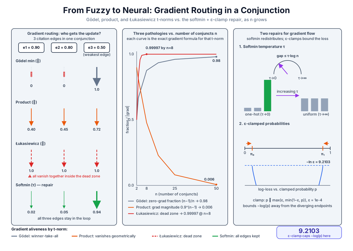Three t-norms, one conjunction, three failure modes as the conjunction grows, and the two repairs: softmin redistributes the gradient as softmax weights, and the ε-clamps bound the log-loss at the boundary. Original diagram by the authors, created with AI assistance.

Gödel min: one winner takes the whole gradient

The Gödel conjunction $T_G(x) = \min_i x_i$ is piecewise linear: on each region of the input space where a particular coordinate is the smallest, $T_G$ coincides with that coordinate exactly. Make that precise. Suppose coordinate $k$ is the unique argmin, meaning $x_k \lt x_j$ for every $j \ne k$. Let $\delta = \tfrac{1}{2}\min_{j \ne k}(x_j - x_k)$, half the smallest gap to any competitor; $\delta$ is strictly positive by uniqueness. Perturb every coordinate by less than $\delta$: coordinate $k$ rises to at most $x_k + \delta$, every other coordinate falls to at least $x_j - \delta \ge x_k + 2\delta - \delta = x_k + \delta$, so coordinate $k$ is still the minimum. On that whole neighborhood, $T_G(x) = x_k$ identically, an equality of functions, and we may differentiate both sides:

$$\frac{\partial T_G}{\partial x_k} = 1, \qquad \frac{\partial T_G}{\partial x_j} = 0 \;\; \text{for every } j \ne k.$$

The gradient of min is the one-hot indicator of the argmin: a vector of zeros with a single 1. At a tie the derivative does not exist ($\min(x, y)$ has a kink along $x = y$), and the standard escape is the supergradient: min is a concave function (one whose graph never dips below its chords, so it has supergradients where a convex function has subgradients), its supergradients at a tie form the convex hull (every weighted average with nonnegative weights summing to one) of the tied coordinates' indicator vectors, and picking one of them (the code picks the first argmin) is a valid choice. (Practitioners often say "subgradient" for the convex and concave cases alike; that colloquial umbrella name is the one the code comment uses.) This is the same convention Volume 3 used at the kinks of its hinge losses in EL Embeddings, and it is safe for the same reason: under any continuous distribution on the inputs, an exact tie has probability zero. The companion does not leave that to faith; it asserts that no tie occurs in any sampled batch (fuzzy_grad.py lines 176–178). The implementation is four lines (fuzzy_grad.py lines 76–83):

def godel_grad(x: np.ndarray) -> np.ndarray:
    # ∂/∂x_i min(x) = 1 if i = argmin(x), else 0.  Away from ties min is
    # locally just its smallest coordinate, so the derivative is the
    # indicator of the argmin (at a tie we take the first-argmin
    # subgradient; ties have probability 0 under continuous sampling).
    g = np.zeros_like(x)
    g[int(np.argmin(x))] = 1.0
    return g

Now name the consequence. In an $n$-way conjunction, exactly $n - 1$ of the $n$ inputs receive gradient zero: they learn nothing this step. The zero-gradient fraction is therefore exactly $(n-1)/n$, and the measured fraction on 2000 seeded uniform batches per $n$ agrees to every printed digit (fuzzy_grad.py lines 168–183):

[2] Gödel (min) gradient SPARSITY — fraction of the n inputs that
    receive zero gradient (2000 seeded uniform batches per n):
    n     zero-grad fraction   exact (n-1)/n
    2               0.5000          0.5000
    5               0.8000          0.8000
    10              0.9000          0.9000
    20              0.9500          0.9500
    50              0.9800          0.9800

At $n = 50$, 98 percent of the conjuncts are starved on any given step. This is what the systematic analysis calls a single-passing gradient [1]: the entire learning signal passes through one input, and every other atom's error, however large, is invisible until the current weakest atom improves enough to hand over the argmin. Training can still make progress (the argmin migrates), but credit assignment is serialized: a fifty-atom rule body is corrected one atom at a time.

Product: every input alive, every gradient shrinking

The product conjunction $T_P(x) = \prod_{j=1}^{n} x_j$ (the symbol $\prod$ multiplies its terms over the index range, as $\sum$ adds them) is smooth everywhere, and its partial derivative is a one-step computation once the product is factored. Isolate coordinate $i$:

$$T_P(x) \;=\; x_i \cdot \underbrace{\prod_{j \ne i} x_j}_{\text{constant in } x_i},$$

where the underbraced factor collects every term except $x_i$ and therefore does not change when $x_i$ does. Differentiating a constant times $x_i$ gives the constant:

$$\frac{\partial T_P}{\partial x_i} \;=\; \prod_{j \ne i} x_j,$$

the leave-one-out product. (The same result follows from the binary product rule $\tfrac{d}{dx}(x \cdot c) = c$ applied inductively, one factor at a time; the factorization argument just does all $n-1$ steps at once.) The implementation is a direct transcription (fuzzy_grad.py lines 91–94):

def prod_grad(x: np.ndarray) -> np.ndarray:
    # ∂/∂x_i ∏_j x_j = ∏_{j≠i} x_j     (leave-one-out product: differentiate
    # the product treating every other factor as a constant).
    return np.array([float(np.prod(np.delete(x, i))) for i in range(len(x))])

On the running chain this gives $(0.8 \cdot 0.5,\; 0.9 \cdot 0.5,\; 0.9 \cdot 0.8) = (0.40, 0.45, 0.72)$, the row the routing table printed: dense, and sensibly ranked, since the partial with respect to an input omits that input's own value, so the weakest conjunct sees the largest gradient. So far, the product looks like the right answer. The problem is scale. Set every input to the same value $c$, a "mildly true" rule body with all atoms at confidence $c$; the display below writes this constraint as $x_j = c \;\forall j$, where the symbol $\forall$ reads "for every". Then the leave-one-out product is $c$ multiplied by itself $n - 1$ times:

$$\frac{\partial T_P}{\partial x_i}\bigg|_{x_j = c \;\forall j} \;=\; c^{\,n-1} \;=\; e^{(n-1)\log c},$$

where $\log$ is the natural logarithm, the logarithm whose base is the constant $e \approx 2.71828$ of the exponential function $e^x$; it is the inverse of that exponential, so $e^{\log c} = c$, and every logarithm in this chapter, always written $\log$, is this base-$e$ one. Since $\log c \lt 0$ for any $c \lt 1$, this is a geometric decay in the number of conjuncts: each additional atom multiplies every other atom's gradient by $c$. At $c = 0.9$, $\log 0.9 \approx -0.105$, so fifty conjuncts shrink the gradient by a factor of $e^{-49 \times 0.105} \approx e^{-5.16}$. The committed magnitudes (fuzzy_grad.py lines 186–196):

[3] product gradient VANISHING — |∂T_P/∂x_i| = ∏_{j≠i} x_j at
    x_j = 0.9 for all j (a mildly-true n-clause rule body):
    n     |gradient| = 0.9^(n-1)
    2     0.900000
    5     0.656100
    10    0.387420
    20    0.135085
    50    0.005726

By $n = 50$ the gate has closed to below $0.006$: whatever learning rate the optimizer uses, the effective learning rate on each atom of a fifty-atom body is cut by a factor of 175. This is the classic vanishing-gradient disease of deep networks in different clothing: backpropagation multiplies one factor per layer, each typically below one, and the product shrinks geometrically with depth; Volume 3's Attention chapter measured the softmax version of exactly this collapse. Here the multiplication is not through layers of a network but through the conjuncts of a formula: a long rule body is a deep network in the gradient's eyes, and the product t-norm makes its depth explicit [1]. The repair, worked out below, is the standard one for products that vanish: move to log space.

Łukasiewicz: the dead zone

The binary Łukasiewicz conjunction is $T_{\text{Ł}}(x, y) = \max(0, x + y - 1)$. Chaining it by associativity gives a closed form worth deriving, because the gradient story lives entirely inside it. Claim: the $n$-ary left fold equals

$$T_{\text{Ł}}(x_1, \ldots, x_n) \;=\; \max\!\Big(0,\; \sum_{i=1}^{n} x_i - (n-1)\Big).$$

Proof by induction on the number of folded inputs. Write $F_k$ for the fold after $k$ inputs, and suppose $F_k = \max\big(0, \sum_{i \le k} x_i - (k-1)\big)$; the base case $F_1 = x_1$ holds because a sum of one term minus zero is $x_1$, which is nonnegative. The next fold step is $F_{k+1} = \max(0, F_k + x_{k+1} - 1)$. Two cases. If $F_k \gt 0$, then $F_k = \sum_{i \le k} x_i - (k-1)$, and substituting gives $F_{k+1} = \max\big(0, \sum_{i \le k+1} x_i - k\big)$, the claimed form. If $F_k = 0$, the hypothesis says $\sum_{i \le k} x_i \le k - 1$; adding $x_{k+1} \le 1$ to both sides gives $\sum_{i \le k+1} x_i \le k$, so $\sum_{i \le k+1} x_i - k \le 0$ and the claimed form evaluates to $\max(0, \text{something} \le 0) = 0$, while the fold step gives $\max(0, 0 + x_{k+1} - 1) = 0$ as well, since $x_{k+1} \le 1$. Both cases agree. ∎ The companion checks this identity against fifty random folds of random arity (fuzzy_grad.py lines 271–277).

Now differentiate the closed form. Write $s = \sum_i x_i - (n-1)$, the pre-clamp value. Where $s \gt 0$, the max is inactive and $T_{\text{Ł}} = s$, a linear function whose slope in every coordinate is 1:

$$\frac{\partial T_{\text{Ł}}}{\partial x_i} = 1 \quad \text{for every } i \qquad (s \gt 0).$$

Where $s \lt 0$, the clamp is active and $T_{\text{Ł}} \equiv 0$ on a whole neighborhood, a constant function:

$$\frac{\partial T_{\text{Ł}}}{\partial x_i} = 0 \quad \text{for every } i \qquad (s \lt 0),$$

with the subgradient 0 chosen at the kink $s = 0$, the same hinge convention as before (fuzzy_grad.py lines 104–109). Notice how different this is from min's failure. Min starves $n-1$ inputs but always teaches one. Łukasiewicz is all-or-nothing per example: either every conjunct gets slope 1 (the routing table's row, because the chain's sum $0.9 + 0.8 + 0.5 = 2.2$ just clears the threshold $n - 1 = 2$), or every conjunct gets exactly 0. The region where everything dies, the dead zone, is the set $\lbrace x \in [0,1]^n : \sum_i x_i \le n - 1 \rbrace$; read the braces aloud as "the set of points $x$ in the $n$-dimensional unit cube such that the coordinates of $x$ sum to at most $n - 1$" (the colon means "such that"). Its size is not a matter of opinion; it has an exact volume.

Substitute $u_i = 1 - x_i$, each $u_i$ the doubt of conjunct $i$. The map $x \mapsto u$ (read the arrow $\mapsto$ aloud: $x$ is sent to $u$) is a reflection of the unit cube onto itself, so it preserves volume, and if $x$ is uniform on the cube then so is $u$. The alive condition transforms as follows (the double arrow $\Longleftrightarrow$ reads "exactly when": each line of the chain holds precisely when the next one does)

$$\sum_i x_i \gt n - 1 \;\Longleftrightarrow\; \sum_i (1 - u_i) \gt n - 1 \;\Longleftrightarrow\; n - \sum_i u_i \gt n - 1 \;\Longleftrightarrow\; \sum_i u_i \lt 1 :$$

the conjunction is alive exactly when the total doubt is under one. The alive region is the standard simplex corner $\lbrace u \ge 0,\; \sum_i u_i \lt 1\rbrace$, whose volume we now derive. Let $V_n(t)$ be the volume of $\lbrace u \in [0,\infty)^n : \sum_i u_i \le t \rbrace$ for $t \in [0,1]$ (staying inside the cube because each $u_i \le t \le 1$). Claim: $V_n(t) = t^n / n!$, where $n! = n \cdot (n-1) \cdots 2 \cdot 1$ is the factorial. Base case: $V_1(t) = t$, the length of the interval $[0, t]$, and $t^1/1! = t$. Inductive step: slice along the last coordinate, writing $w$ for the slice height (a fresh letter, so it cannot be confused with the pre-clamp value $s$ above). If $u_n = w$, the remaining coordinates must satisfy $\sum_{i \lt n} u_i \le t - w$, a set of volume $V_{n-1}(t - w)$, so

$$V_n(t) \;=\; \int_0^t V_{n-1}(t - w)\, dw \;=\; \int_0^t \frac{(t-w)^{n-1}}{(n-1)!}\, dw \;=\; \int_0^t \frac{r^{n-1}}{(n-1)!}\, dr \;=\; \frac{t^n}{n\,(n-1)!} \;=\; \frac{t^n}{n!},$$

where the middle step substitutes $r = t - w$ (so $dr = -dw$ and the limits flip, canceling the sign). At $t = 1$ the alive probability is $1/n!$, so the dead fraction of a uniform random input is $1 - 1/n!$, and factorials grow brutally: $1 - 1/24 \approx 0.958$ at $n = 4$, $1 - 1/40320 \approx 0.99998$ at $n = 8$. The measurement on 200,000 uniform samples per $n$ (fuzzy_grad.py lines 199–213):

[4] Łukasiewicz DEAD ZONE — max(0, Σx-(n-1)) clamped at 0 gives
    ZERO gradient to every input; dead fraction of 200,000 uniform
    samples vs the exact simplex volume 1 - 1/n!:
    n     measured    exact 1-1/n!
    2     0.50050     0.50000
    3     0.83271     0.83333
    4     0.95878     0.95833
    5     0.99177     0.99167
    8     0.99997     0.99998

Read the last row as a verdict: initialize a network whose predicate outputs are anywhere near uniform, conjoin eight of them with Łukasiewicz, and 99.997 percent of examples contribute nothing to the gradient. Beyond $n \approx 4$, essentially nothing trains unless the inputs are already close to true [1], which is why the practical workaround for this t-norm is warm-started truths or short conjunctions.

Softmin: the smooth repair

Min's problem is that its gradient is a one-hot vector. The repair is to replace the hard minimum with a smooth function that converges to min while spreading its gradient over every input. The standard construction is softmin, the log-sum-exp smoothing: for a temperature $\tau \gt 0$ (a knob with the units of the inputs; small $\tau$ means sharp, large $\tau$ means smooth),

$$\operatorname{softmin}_\tau(x) \;=\; -\tau \,\log \sum_{i=1}^{n} e^{-x_i/\tau}.$$

Decode the construction from the inside out: dividing by $\tau$ and negating turns small truth degrees into large exponents, the exponentials make the smallest $x_i$ dominate the sum, the log undoes the exponential scale, and the outer $-\tau$ undoes the negation and the division. Two limits pin down its behavior, and both are short derivations.

Small τ: softmin converges to min, with an explicit gap bound. Let $m = \min_i x_i$. Factor $e^{-m/\tau}$ out of the sum:

$$\sum_{i=1}^{n} e^{-x_i/\tau} \;=\; e^{-m/\tau} \sum_{i=1}^{n} e^{-(x_i - m)/\tau}.$$

In the shifted sum every exponent $-(x_i - m)/\tau$ is at most 0 (because $x_i \ge m$), so every term is at most $e^0 = 1$ and the sum is at most $n$; and the argmin's own term is exactly $e^0 = 1$, so the sum is at least 1. Take logarithms, which preserve order: $0 \le \log \sum_i e^{-(x_i-m)/\tau} \le \log n$. Now apply $-\tau \log(\cdot)$ to the factored product; the log of a product is the sum of logs, so

$$\operatorname{softmin}_\tau(x) \;=\; -\tau\Big({-\tfrac{m}{\tau}} + \log \sum_i e^{-(x_i-m)/\tau}\Big) \;=\; m - \tau \log \sum_i e^{-(x_i - m)/\tau},$$

and substituting the bracket's bounds (multiplying by $-\tau$ flips them):

$$m - \tau \log n \;\le\; \operatorname{softmin}_\tau(x) \;\le\; m.$$

Softmin approaches min from below, and its gap is at most $\tau \log n$, linear in the temperature. Halve $\tau$ and the worst-case gap halves. The factored form is also how the code computes it without overflow: the shifted exponents are all nonpositive, so nothing explodes even at $\tau = 0.01$ (fuzzy_grad.py lines 114–124).

Large τ: softmin flattens toward the mean. Expand each exponential to first order, $e^{-x_i/\tau} = 1 - x_i/\tau + O(1/\tau^2)$ (the notation $O(1/\tau^2)$ collects terms that shrink at least as fast as $1/\tau^2$). Summing over $i$ and writing $\bar{x} = \tfrac{1}{n}\sum_i x_i$ for the arithmetic mean, the sum is $n\big(1 - \bar{x}/\tau + O(1/\tau^2)\big)$. Using $\log(ab) = \log a + \log b$ and $\log(1 + z) = z + O(z^2)$,

$$\operatorname{softmin}_\tau(x) \;=\; -\tau\Big(\log n - \frac{\bar{x}}{\tau} + O(1/\tau^2)\Big) \;=\; \bar{x} - \tau \log n + O(1/\tau).$$

Up to the input-independent offset $\tau \log n$, a hot softmin is just the average of its inputs: no input is special, which is the flat end of the dial. The interesting end for training is the gradient, and it has a name. One more rule is needed first, the derivative of the natural logarithm: for $u \gt 0$, $\tfrac{d}{du}\log u = \tfrac{1}{u}$, so the rate of change of $\log u$ is the reciprocal of its argument (differentiate the identity $e^{\log u} = u$ by the chain rule to get $e^{\log u} \cdot \tfrac{d}{du}\log u = 1$, then divide both sides by $e^{\log u} = u$); the log-space losses later in the chapter lean on the same rule. With $S = \sum_j e^{-x_j/\tau}$, the chain rule gives, step by step,

$$\frac{\partial}{\partial x_i}\big(-\tau \log S\big) \;=\; -\tau \cdot \frac{1}{S} \cdot \frac{\partial S}{\partial x_i} \;=\; -\tau \cdot \frac{1}{S} \cdot e^{-x_i/\tau} \cdot \Big({-\frac{1}{\tau}}\Big) \;=\; \frac{e^{-x_i/\tau}}{S} \;=\; \operatorname{softmax}(-x/\tau)_i .$$

The gradient of softmin is exactly the softmax weight vector of the negated, temperature-scaled inputs: each component is strictly positive (an exponential is never zero) and they sum to $S/S = 1$, a convex combination. Every conjunct stays alive on every step, and the temperature dials the sparsity continuously: as $\tau \to 0$ the weights concentrate onto the argmin (recovering Gödel's one-hot routing as a limit), and as $\tau \to \infty$ they flatten to the uniform vector $(1/n, \ldots, 1/n)$. The implementation, with the same overflow-safe shift, which cancels in the ratio (fuzzy_grad.py lines 127–134):

def softmin_grad(x: np.ndarray, tau: float) -> np.ndarray:
    # With S = Σ_j exp(-x_j/τ):
    #   ∂softmin/∂x_i = -τ · (1/S) · exp(-x_i/τ) · (-1/τ)
    #                 = exp(-x_i/τ) / S  =  softmax(-x/τ)_i.
    # Every weight is strictly positive and they sum to 1: a convex
    # combination that leans on the smallest inputs but starves none.
    z = np.exp(-(x - float(np.min(x))) / tau)   # same shift, cancels in z/Σz
    return z / float(np.sum(z))

On the running chain at $\tau = 0.1$ the weights are $(0.0171, 0.0466, 0.9362)$: the weakest edge still receives 94 percent of the gradient, min-like behavior, but the other two edges receive real, nonzero signal, and the finite-difference check certifies the derivation to $1.064 \times 10^{-11}$. The convergence claim is likewise a committed table, not a limit argument left in the abstract (fuzzy_grad.py lines 216–226): the maximum gap over 500 uniform vectors in $[0,1]^5$ shrinks with $\tau$ and always respects the bound $\tau \log 5 \approx 1.609\,\tau$:

[5] softmin_τ(x) = -τ·log Σ exp(-x_i/τ): the smooth min —
    max |softmin_τ - min| over 500 uniform vectors (n = 5):
    τ       max gap     bound τ·log n
    1.0     1.544452    1.609438
    0.1     0.119991    0.160944
    0.01    0.006536    0.016094

The boundary explosion and the ε-clamps

Softmin repairs min. The product's vanishing has its own classical repair: work in log space. Maximizing $T_P(a) = \prod_i a_i$ over the truth vector $a = (a_1, \ldots, a_n)$ of a batch of groundings is the same as minimizing its negative log, because the logarithm is strictly increasing:

$$L(a) \;=\; -\log \prod_{i=1}^{n} a_i \;=\; -\sum_{i=1}^{n} \log a_i, \qquad \frac{\partial L}{\partial a_i} \;=\; -\frac{1}{a_i}.$$

Compare that partial to the leave-one-out product. The log has decoupled the conjuncts: atom $i$'s gradient depends only on its own truth value, with no product over the other $n - 1$ factors, so nothing vanishes as $n$ grows. Weak atoms (small $a_i$) get large corrective gradients, strong atoms get small ones. This log-product loss is the repair the systematic operator analysis itself recommends for exactly this job of aggregating a batch of groundings, and the decoupled $1/a_i$ derivative is derived there [1]. Logic Tensor Networks (LTN) works in the same product family but keeps its loss in truth space: its production default, the stable product configuration, pairs the product-family connectives with generalized p-mean aggregators for the quantifiers (power means with a tunable exponent), guards every singular input with the projections introduced below, and trains on the loss $1 - \mathrm{SatAgg}$, one minus the aggregated satisfaction of the theory [2]. Log loss or truth-space loss, the singularity sits at the boundary of the truth interval, exactly where real data puts it. As $a_i \to 0$ the loss term $-\log a_i$ diverges and the gradient magnitude $1/a_i$ is unbounded. The mirrored loss for a negated formula, $-\log(1 - a_i)$, diverges the same way as $a_i \to 1$.

The companion builds the exhibit from the running world (fuzzy_grad.py lines 310–325): the truth vector $a = (1.0,\; 0.9,\; 0.0)$, where 1.0 is the crisply asserted fact advises(alice, bob) from Volume 1's kb.py, 0.9 is cites(p3, p2) from Volume 2's annotated.py, and 0.0 is the reversed edge cites(p1, p3), which is simply false. One exactly-false grounding, and the whole conjunction loss $-\sum_i \log a_i$ is literally infinite; one exactly-true grounding, and the negation loss $-\log(1 - a)$ is infinite too. A single confident example destroys the entire batch's update. The repair is a pair of affine stability projections with a small constant $\varepsilon$ (the code uses $\varepsilon = 10^{-4}$, fuzzy_grad.py line 66), applied to a truth value before it enters a log or a quotient (fuzzy_grad.py lines 139–148):

def pi_0(a, eps: float = EPS):
    # π₀(a) = (1-ε)·a + ε   — maps [0,1] to [ε, 1]: bounds truth values away
    # from 0 before a log/quotient that is singular there (LTN eq. 13/19).
    return (1.0 - eps) * a + eps


def pi_1(a, eps: float = EPS):
    # π₁(a) = (1-ε)·a       — maps [0,1] to [0, 1-ε]: bounds truth values
    # away from 1 before log(1-a) etc. (LTN eq. 14/20).
    return (1.0 - eps) * a

π₀ compresses the unit interval into $[\varepsilon, 1]$, pulling truth values off the floor; π₁ compresses it into $[0, 1-\varepsilon]$, pulling them off the ceiling. Both bounds now follow by the chain rule, every step shown. For the positive side, $\pi_0'(a) = 1 - \varepsilon$ (the derivative of an affine function is its slope), so

$$\frac{d}{da}\big[-\log \pi_0(a)\big] \;=\; -\frac{\pi_0'(a)}{\pi_0(a)} \;=\; -\frac{1-\varepsilon}{\pi_0(a)}, \qquad \Big|\frac{d}{da}\big[-\log \pi_0(a)\big]\Big| \;\le\; \frac{1-\varepsilon}{\varepsilon},$$

the last step because $\pi_0(a) \ge \varepsilon$ everywhere on $[0,1]$. The loss itself obeys $-\log \pi_0(a) \le -\log \varepsilon$ for the same reason. For the negation side, $1 - \pi_1(a) = 1 - (1-\varepsilon)a \ge 1 - (1-\varepsilon) = \varepsilon$, and

$$\frac{d}{da}\big[-\log(1 - \pi_1(a))\big] \;=\; \frac{\pi_1'(a)}{1 - \pi_1(a)} \;=\; \frac{1-\varepsilon}{1 - \pi_1(a)} \;\le\; \frac{1-\varepsilon}{\varepsilon}.$$

With $\varepsilon = 10^{-4}$ the ceilings evaluate to $-\log \varepsilon = 9.2103$ per loss term and $(1-\varepsilon)/\varepsilon = 9999.0$ per gradient: large, still steering hard toward the constraint, but finite. Both clamp derivatives receive the same certification as the four connective gradients: the analytic forms $-(1-\varepsilon)/\pi_0(a)$ and $(1-\varepsilon)/(1-\pi_1(a))$ are checked against the central finite difference at the smooth chain point (fuzzy_grad.py lines 344–354). The committed with/without exhibit (fuzzy_grad.py lines 330–343):

[6] the LTN stability clamps π₀(a) = (1-ε)a + ε, π₁(a) = (1-ε)a
    (ε = 0.0001); grounding truths a = (1.0, 0.9, 0.0):
    advises(alice,bob) = 1.0 (crisp fact, kb.py), cites(p3,p2) =
    0.9 (annotated.py), reversed cites(p1,p3) = 0.0 (false).
                                unclamped        with π₀/π₁
    -Σ log a_i  (∧ as loss)     inf              9.3157
    max |∂| = 1/a               inf              9999.0
    -log(1-a) at a = 1 (¬φ)     inf              9.2103
    ∂ = 1/(1-a)                 inf              9999.0
    bounds with clamps: loss ≤ -log ε = 9.2103 per term, |grad| ≤ (1-ε)/ε = 9999.0
    one exactly-false grounding turns the whole loss to inf — the
    clamps are load-bearing, not cosmetic (LTN eqs. 19-20).

State the price as plainly as the benefit, because the source system does [2]. A clamped conjunction is no longer exactly a t-norm. Push the projection through the product and consider the effective binary connective $\tilde{T}(x, y) = \pi_0(x) \cdot \pi_0(y)$: setting $y = 1$, and noting $\pi_0(1) = (1-\varepsilon)\cdot 1 + \varepsilon = 1$, gives $\tilde{T}(x, 1) = \pi_0(x) \cdot 1 = (1-\varepsilon)x + \varepsilon \ne x$, so the unit law $T(x, 1) = x$, the axiom the last chapter verified with deviation exactly 0.0, now fails by up to $\varepsilon$. The trade is deliberate: a bounded loss and a bounded gradient, purchased with a small, permanent distortion of the algebra.

The design table

One table now summarizes the chapter, and later chapters reuse it whenever a system declares its t-norm. Every cell is a committed number from the runs above, not a qualitative impression.

conjunction	$\partial T / \partial x_i$	gradient character	measured failure at scale	repair
Gödel $\;T_G = \min_i x_i$	1 on the argmin, else 0	sparse: single-input credit assignment	zero-gradient fraction $0.9800$ at $n = 50$	softmin$_\tau$: all weights positive, gap $\le \tau \log n$ (measured $0.006536$ at $\tau = 0.01$, $n = 5$)
product $\;T_P = \prod_i x_i$	$\prod_{j \ne i} x_j$	dense, sensibly ranked, but shrinking	$0.9^{49} = 0.005726$ at $n = 50$	log space ($\partial = -1/a_i$, no leave-one-out product) plus π₀/π₁ clamps (loss $\le 9.2103$ per term, gradient $\le 9999.0$)
Łukasiewicz $\;T_{\text{Ł}} = \max(0, \sum_i x_i - (n-1))$	1 for every input if $\sum_i x_i \gt n-1$, else 0 for every input	binary: all alive or all dead	dead fraction $1 - 1/n!$, measured $0.99997$ at $n = 8$	keep conjunctions short, warm-start truths near 1, or avoid it for long bodies

These are not hypothetical menu choices. Constrained training losses built from exactly these three t-norms have been compared head to head on a real perception task with logical requirements, the ROAD-R autonomous-driving benchmark, where the t-norm is an explicit design axis of the loss [3]. And this fuzzy family, truth-functional operators made differentiable, with the gradient as the design criterion, is one branch of a larger map of neuro-symbolic methods; the survey of that landscape places it beside the probabilistic family that Part II of this volume turns to next [4].

The unsolved part

Every repair in this chapter buys trainability by selling algebra, and the debt can be computed exactly. Softmin is not a t-norm. Feed it the unit element: with two inputs $x$ and $1$,

$$\operatorname{softmin}_\tau(x, 1) \;=\; -\tau \log\big(e^{-x/\tau} + e^{-1/\tau}\big) \;\lt\; -\tau \log\big(e^{-x/\tau}\big) \;=\; x,$$

the strict inequality because the sum inside the log has a second, strictly positive term and the outer $-\tau\log(\cdot)$ is strictly decreasing. So the unit law $T(x, 1) = x$, the axiom the previous chapter verified with deviation exactly 0.0, fails for every $x$ and every $\tau \gt 0$. Worse, softmin does not even stay inside the truth interval: at the corner $x = (1, 1)$ it returns $1 - \tau \log 2$, and at $(0, 0)$ it returns $-\tau \log 2$, a negative truth value ($\approx -0.069$ at $\tau = 0.1$). The ε-clamps carry the same kind of debt, quantified at the end of the previous section: the clamped product violates the unit law by up to $\varepsilon$, permanently. None of this is hidden by the systems that use these repairs; the stable product configuration is documented precisely as a numerical necessity rather than a logical choice [2]. What remains genuinely open is the audit. A trained model's loss curve reports the smoothed logic (softmin at the training temperature, clamped truths), while the semantics the practitioner reasons about, and reports results in, is the un-smoothed t-norm. No current framework tracks the gap between the two: how far the formula truths a system certifies at $\tau = 0.1$ can drift from the truths min would assign, accumulated over thousands of formulas and training steps, is measured in this chapter for one conjunction (at most $\tau \log n$ per application, by the sandwich bound) and audited nowhere at scale. Trainability is bought with logical debt, and the field currently keeps no ledger.

Why it matters

This chapter is the volume's hinge in miniature. Part I's promise was that logic could become a loss; the routing table is the fine print of that promise. Every differentiable-logic system that follows must declare a conjunction, and the moment it does, it inherits a row of the design table: the Logic Tensor Networks chapter builds an entire language on the stable product configuration whose clamps were priced here, the Semantic Loss chapter keeps the product but reroutes it through exact probability, and the fuzzy query-answering machinery late in the volume runs Gödel and product operators over millions of embedded atoms, where the difference between a one-hot gradient and a softmax gradient decides what trains at all. The chapter also closes a loop with the series' two pillars. The symbolic pillar contributed the operators and their axioms; the neural pillar contributed the one question axioms never ask, what is your derivative, and the vanishing-gradient disease that Volume 3's Attention chapter measured in its softmax form turned out to apply verbatim to a fifty-atom rule body. Looking ahead to Volume 5, the lesson generalizes into a trust question: a training signal that silently starves 98 percent of its atoms, or dies on 99.997 percent of its examples, cannot be diagnosed from the loss curve alone. Auditing what a system actually learned, rather than what its objective claimed to teach, is that volume's opening problem.

Key terms

• Gradient gate: the factor $\partial T / \partial x_i$ that multiplies every parameter update flowing to atom $i$ through a connective; if it is zero, the atom learns nothing this step regardless of its error.
• Single-passing (one-hot) gradient: Gödel min's routing policy, derived from piecewise linearity: derivative 1 on the unique argmin (a supergradient at a tie), 0 on the other $n-1$ inputs, so the zero-gradient fraction is exactly $(n-1)/n$.
• Leave-one-out product: the product t-norm's partial $\partial T_P / \partial x_i = \prod_{j \ne i} x_j$; dense and sensibly ranked, but equal to $c^{\,n-1}$ on uniform inputs, a geometric decay in the number of conjuncts.
• Dead zone: the region $\sum_i x_i \le n - 1$ where the n-ary Łukasiewicz conjunction is clamped at 0 and every input receives exactly zero gradient; its volume under uniform inputs is $1 - 1/n!$, derived from the simplex volume $t^n/n!$.
• Softmin (log-sum-exp smoothing): $\operatorname{softmin}_\tau(x) = -\tau \log \sum_i e^{-x_i/\tau}$; sandwiched between $\min(x) - \tau\log n$ and $\min(x)$, with gradient equal to the softmax weights $\operatorname{softmax}(-x/\tau)$, strictly positive and summing to one.
• Temperature $\tau$: softmin's sharpness dial; $\tau \to 0$ recovers min and its one-hot routing, large $\tau$ flattens toward the mean with uniform weights.
• Stability projections π₀, π₁: the affine clamps $\pi_0(a) = (1-\varepsilon)a + \varepsilon$ and $\pi_1(a) = (1-\varepsilon)a$ that pull truth values off 0 and 1, bounding the log-loss by $-\log\varepsilon$ per term and its gradient by $(1-\varepsilon)/\varepsilon$.
• Stable product configuration: the production recipe of Logic Tensor Networks: product-family operators and generalized p-mean aggregators, with every singular input guarded by a projection; the log-space loss is the companion repair recommended by the systematic operator analysis, guarded by the same projections.
• Central finite difference: the two-sided estimate $\big(f(x + h e_i) - f(x - h e_i)\big)/(2h)$ with error of order $h^2$; the certification tool every hand-derived gradient in this chapter is checked against.
• Logical debt: the semantic distortion a trainability repair introduces (softmin's broken unit law and out-of-range values, the clamps' $\varepsilon$-violation of the unit axiom), traded deliberately for bounded, non-vanishing gradients.

Where this leads

Part I is now complete, and its ledger has two columns. Truth-functional fuzzy logic made every connective a fixed, cheap, differentiable function, and this chapter showed the price: the honest operators have pathological gradients, and the trainable operators are no longer quite logic. Part II takes the other branch of the map [4]. It abandons truth-functionality altogether: the probability of a conjunction is not a function of the probabilities of its conjuncts (it depends on how the conjuncts share evidence), so no table of operators, however cleverly smoothed, can compute it. The replacement is the distribution semantics, in which a logic program with probabilistic facts defines a single, exact distribution over possible worlds, and the truth of a query is a genuine probability with a genuine, well-behaved derivative. The calculus becomes exact; nothing is clamped, nothing is smoothed, and no unit law is broken. The cost moves elsewhere, from gradient pathology to counting, because summing over possible worlds is exponential work that must be tamed by compilation. The next chapter, Distribution Semantics, builds that foundation on the same academic-world knowledge base, turning eleven of its twenty-three facts into independent coins, and the two chapters after it pay the counting bill.

---

Companion code: examples/integration/fuzzy_grad.py implements every operator, every hand-derived gradient, the finite-difference certifier, and all four measurement studies in this chapter; the t-norm algebra it differentiates is the one examples/integration/tnorms.py verified exactly in the previous chapter. Run python3 fuzzy_grad.py from examples/integration/ to reproduce every table above; the suite harness examples/integration/validate.py re-executes its asserts (the routing vector, the FD gates, the $(n-1)/n$ sparsity law, the $0.9^{49}$ vanishing floor, the $1 - 1/n!$ dead-zone match, the $\tau\log n$ bound, and the clamp bounds) as part of the volume's acceptance verdict.