Fuzzy and Training-Free CLQA: CQD, GNN-QE, QTO

📍 Where we are: Part V · Complex Logical Query Answering — Chapter 17. From GQE to BetaE answered complex queries by learning a new geometry per query structure, trained on sampled multi-hop queries; this chapter deletes that training and asks whether one calibrated 1-hop predictor, composed by fuzzy logic, already suffices.

The query-embedding line of the previous chapter carries a hidden bill. GQE (Graph Query Embedding), Query2Box, and BetaE each learn query-level parameters: intersection networks, box offsets, Beta-distribution operators, all fit by gradient descent on millions of sampled query-answer pairs, one training distribution per query structure. Miss a structure at training time and the model has never seen its shape. This chapter develops the opposing thesis: the knowledge a complex query needs is already in the 1-hop predictor, and everything above the atoms is inference, not learning. Calibrate the link predictor's scores into truth values between 0 and 1, and Part I's fuzzy connectives do the rest: a conjunction is a product, an existential quantifier is a maximization, and a whole query becomes an optimization problem that its computation graph organizes. We run that thesis three ways on the academic world: greedily (the beam search of CQD, Continuous Query Decomposition, over concrete entities), densely (the fuzzy-set reading that keeps a membership score for all 13 entities at every node), and exactly (the dynamic program of QTO, Query Computation Tree Optimization, over the query tree, which returns the provable optimum together with a checkable proof).

The simple version

Imagine planning a two-leg trip with a reliability table: for every pair of cities, a number between 0 and 1 saying how dependable the direct connection is. Nobody retrains a special "two-leg model." A two-leg trip through a layover city is as dependable as its weaker legs make it (multiply the two numbers), and the best layover is whichever city maximizes that product. A hurried planner shortlists the four most promising layovers and ignores the rest: fast, but if the true best layover missed the shortlist, no later cleverness recovers it. A careful planner keeps a running score for every city on the map, so nothing is ever discarded. And a patient planner with a big enough spreadsheet computes the exact best itinerary and hands you the receipt: these two legs, with these two reliabilities, multiply to exactly this score. Those three planners are CQD-Beam, the fuzzy-set executor, and QTO, and the reliability table is the calibrated 1-hop predictor they all share.

What this chapter covers

• The provocation, quantified: the previous chapter's models train on sampled complex queries; CQD's claim is a pretrained 1-hop predictor plus t-norm composition, with zero query-level training, which reframes complex-query competence as an inference property rather than a learning property.
• The atom layer, built carefully: Volume 3's ComplEx retrained on the 15 observed edges, then calibrated into a neural adjacency matrix $M_r \in [0,1]^{13 \times 13}$ (per relation $r$, a 13-by-13 grid of truth values between 0 and 1, decoded fully in the atom-layer section) by a per-row softmax recipe, with every observed edge pinned to exactly 1 and every imputed entry capped strictly below 1.
• The query as fuzzy optimization: conjunction as the product t-norm, the existential quantifier as a max over 13 candidate bindings, negation as the complement where the language supports it; the 2p query's full objective written and decoded symbol by symbol.
• Three executors, one algebra: CQD-Beam's top-k concrete entities (interpretable, greedy, and derivably lossy), the full membership vector that prunes nothing, and QTO's exact max-product dynamic program, with the derivation of why trees admit exact DP.
• A faithful proof: the backward argmax pass that extracts the witnessing assignment, quoted from the committed run and checked edge by edge, including the corollary-in-miniature that provable answers are never missed because they ride pinned-to-1 edges.
• The committed three-way table: symbolic traversal at a hard-answer MRR (mean reciprocal rank) of 0.1465, both training-free answerers at 0.8000, the oracle at 1.0000, and the honest reading of where the remaining 0.2 went.
• The honest phrase: "training-free" holds at the query level only; the 1-hop predictor is still trained, and its calibration silently bounds everything downstream.

The provocation: competence without query-level training

State the previous chapter's cost model precisely. A query-embedding system must learn parameters for every operator its query language contains, and those parameters are fit on sampled complex queries: the standard pipeline mines hundreds of thousands of query instances of each structure (1p, 2p, 2i, and the rest), millions in total, from the training graph and runs contrastive gradient descent on all of them, the training bill the previous chapter quantified and cited against the standard benchmarks in its closing section. The training set is not the knowledge graph anymore; it is a synthetic distribution over query shapes, and generalization to an unseen shape is an empirical gamble.

CQD makes the opposing bet [1]: train nothing beyond the 1-hop link predictor that Volume 3 already built. Every complex query is assembled from atoms of the form $r(a, x)$, "entity $a$ relates to candidate $x$ through relation $r$", and a 1-hop predictor already assigns every such atom a score. What is missing is not knowledge but composition: a principled way to combine atom scores across conjunctions and existential quantifiers. Part I of this volume built exactly that machinery; the t-norms chapter showed how a t-norm turns pairs of truth values in $[0,1]$ into the truth value of their conjunction. So the recipe is: squash atom scores into $[0,1]$, compose them with a t-norm, and read the query as an optimization problem over the unknown variables. No intersection network, no box offsets, no Beta parameters. If this works even approximately as well as the trained geometries, then complex-query answering is an inference property of a good link predictor, not a learning property of a query encoder, and the whole of Part V pivots on that reframing.

The claim is checkable at our scale because the testbed never changes: the same 13-entity, 5-relation academic world, the same 15-edge training graph with 3 held-out edges, and the same easy/hard answer protocol that query_dag.py fixed earlier in this Part (easy answers are reachable by traversing observed edges; hard answers require imputing a held-out edge, so traversal scores zero on them by definition). The companion module cqd.py runs the entire argument end to end.

The atom layer: from scores to calibrated truths

Everything begins with the reuse. The 1-hop predictor is not a new model; it is Volume 3's ComplEx, retrained byte-identically from the same seed, on the training split only (cqd.py lines 304–306):

    # -- 1-hop ComplEx, retrained exactly as in the Volume 3 suite (seed 0).
    e_re, e_im, w_re, w_im, snaps = bilinear.train_complex(seed=0)
    S = complex_score_table(e_re, e_im, w_re, w_im)

Here bilinear.train_complex is the exact training loop of bilinear.py lines 256–287 (16 real dimensions read as 8 complex, logistic loss, one uniform negative per positive, 1000 epochs), and complex_score_table (cqd.py lines 77–96) evaluates the trained scoring function on every combination at once, giving a raw score tensor $S[r, h, t]$ indexed by the relation $r$, the head entity $h$, and the tail entity $t$. The module spot-checks all $5 \times 13 \times 13 = 845$ entries of this table against bilinear.complex_score, one triple at a time, and asserts the largest discrepancy is below $10^{-9}$ (cqd.py lines 307–312), so every number downstream is the trained model's own opinion, not a re-implementation's.

Raw scores cannot be truth values. A ComplEx score is an unbounded real number: the logistic training loss only pushes positive triples above zero and negatives below, so scores of 3.2 and 5.1 are both "true-ish" with no upper bound, and only their order is meaningful for ranking. The product t-norm needs more than order. For inputs in $[0,1]$ the product satisfies the defining sanity law of conjunction: since $y \le 1$ implies $x \cdot y \le x \cdot 1 = x$, and symmetrically $x \cdot y \le y$, a conjunction is never more true than its weakest conjunct. Feed the product raw scores instead and the law dies: $3.2 \times 5.1 = 16.32$, a "conjunction" more confident than either conjunct. Composition therefore demands calibration: a monotone map from raw scores to $[0,1]$ that preserves the predictor's ranking while giving the outputs a truth-value scale.

The committed calibration is the recipe of QTO [2], implemented in neural_adjacency (cqd.py lines 99–128). Decode it before reading the code. Fix a head entity $h$ and a relation $r$, and look at the row of raw scores over all candidate tails. The softmax of that row, $\exp(S[r,h,t]) / \sum_{e \in V} \exp(S[r,h,e])$, exponentiates each score (making everything positive) and divides by the row's total, so the row becomes a probability-like vector summing to 1; here $V$ is the entity set and $\sum_{e \in V}$ reads "summed over all 13 candidate tails". But a head may truly have several tails (bob advises more than one student), and a vector that sums to 1 cannot say "two of these are fully true". So the recipe rescales the row by $N_t$, the number of tails observed for $(h, r)$ in the training graph (floored at 1 so rows with no observed tail are not zeroed out). Finally two clamps give the matrix its logical teeth: every entry is capped at $1 - \delta$ with $\delta = 10^{-4}$, so no imputed edge can ever reach truth value 1, and then every observed training edge is pinned to exactly 1:

    # Observed tails per (head, relation), from the TRAIN graph only.
    n_tails = np.zeros((N_R, N_E))
    for h, r, t in kg.TRAIN:
        n_tails[kg.R_ID[r], kg.E_ID[h]] += 1.0
    # exp(S) / Σ_tails exp(S), computed stably by shifting each row's max.
    ex = np.exp(S - S.max(axis=2, keepdims=True))
    softmax = ex / ex.sum(axis=2, keepdims=True)
    # r̂ = softmax · N_t  (N_t floored at 1), then the 1-δ cap.
    rhat = softmax * np.maximum(n_tails, 1.0)[:, :, None]
    M = np.minimum(rhat, 1.0 - DELTA)
    # Pin: (e_i, r, e_j) ∈ TRAIN  ⇒  M_r[i,j] = 1 exactly.
    for h, r, t in kg.TRAIN:
        M[kg.R_ID[r], kg.E_ID[h], kg.E_ID[t]] = 1.0
    return M

The result is the neural adjacency matrix: for each relation $r$, a matrix $M_r \in [0,1]^{13 \times 13}$ (read: a 13-by-13 grid of numbers between 0 and 1, one row per head entity, one column per candidate tail) whose entry $M_r[h,t]$ is the calibrated truth of the atom $r(h,t)$. It is the fuzzy generalization of the crisp adjacency matrix a graph algorithm would use: observed edges are exactly 1, everything else is the model's graded guess, strictly below 1. The committed run prints the row that matters most for our running queries:

[1] the neural adjacency M_r (QTO Eq. 3-4 over the trained ComplEx)
  calibration: per (head, r), softmax raw scores over tails, x N_t observed tails,
  cap at 1-delta (delta=0.0001); then every TRAIN edge pinned to exactly 1.0
  15 pinned entries (the 15 TRAIN edges); largest imputed entry 0.9999
  row M[advises][bob, :] — how the model imputes bob's advisees:
    carol    1.000000   pinned: TRAIN edge
    dave     0.000411   imputed: held-out TEST edge
    nesy     0.000005   imputed: not an edge

Read the row as the whole method in miniature. The observed edge (bob, advises, carol) sits at exactly 1.000000 because it was pinned, not because the model earned it. The held-out edge (bob, advises, dave), which the model never saw, is imputed at 0.000411: a small number, but two orders of magnitude above the non-edge (bob, advises, nesy) at 0.000005, and that ratio is what ranking lives on. One honesty note must be posted here and never taken down: every downstream guarantee in this chapter is a guarantee about computing with these numbers, not about the numbers being right. QTO's optimality theorem will find the exact maximizer of the calibrated objective; if the calibration misranks an edge, the exact optimizer inherits the misranking exactly. The committed table at the end of this chapter shows precisely this failure once, and Volume 5's calibration chapter interrogates the question in general.

Composition: the query as a fuzzy optimization problem

Take the running 2p query, in first-order form $q(x) = \exists y.\, \mathrm{advises}(\mathrm{alice}, y) \wedge \mathrm{advises}(y, x)$: "who is advised by an advisee of alice?" Here $x$ is the target variable (the entity being ranked), $y$ is a bound variable (an intermediate entity the query mentions but does not return), $\exists$ reads "there exists", and $\wedge$ reads "and". Under the crisp semantics of the previous chapter, an entity $x$ answers the query when some witness $y$ makes both atoms true edges. The fuzzy semantics replaces each crisp atom with its calibrated truth and each connective with its fuzzy operator, giving every candidate $x$ a graded truth value:

$$T(x) \;=\; \max_{y \in V}\; M_{\mathrm{advises}}[\mathrm{alice}, y] \cdot M_{\mathrm{advises}}[y, x].$$

Decode every piece. $M_{\mathrm{advises}}[\mathrm{alice}, y]$ is the calibrated truth of the first atom with the bound variable set to candidate $y$; the product $\cdot$ is the product t-norm playing $\wedge$, so the grounding's truth is the product of its atoms' truths; and $\max_{y \in V}$, the maximum over all 13 candidate bindings of $y$, plays $\exists$: an existential claim is as true as its best witness makes it. (Max is the standard fuzzy reading of $\exists$, the quantifiers-as-aggregators move the Logic Tensor Networks chapter developed in general; pairing it with the product t-norm from Part I's catalogue for $\wedge$ is what turns query answering into optimization.) The whole query is now a discrete optimization problem: for each target $x$, maximize a product of matrix entries over the assignments of the bound variables. The query's computation DAG (directed acyclic graph), which this Part's opening chapter used to organize crisp set operations, now organizes exactly this optimization: each node carries a vector of truth values over the 13 entities, and each edge applies one fuzzy operator. The full operator menu, with the exact line of cqd.py that implements each:

query node	crisp set semantics (query_dag.py)	fuzzy operator on vectors $v \in [0,1]^{13}$	cqd.py
anchor $e$	the singleton set containing $e$	one-hot vector: $v[e] = 1$, all else 0	lines 167–170
projection by $r$	follow $r$-edges	$v'[t] = \max_h v[h] \cdot M_r[h,t]$	line 189
intersection	set intersection	elementwise product $v = \prod_i v_i$	lines 191–195
union	set union	probabilistic sum $v = 1 - \prod_i (1 - v_i)$	lines 171–176
negation	complement $V - S$	$v' = 1 - v$ (not exercised: the bank is negation-free, EPFO, defined below)	line 179 rejects

Two decoding notes on the table. In the intersection and union rows, $\prod_i$ multiplies over the node's incoming branches $i$, one membership vector $v_i$ per branch. And the committed five-type bank exercises only the anchor, projection, and intersection rows: the union operator is implemented but never called by the committed runs (the exact dynamic program later in this chapter rejects it as unneeded, cqd.py line 221), just as negation is rejected.

EPFO (existential positive first-order) names the negation-free fragment: queries built from $\exists$, $\wedge$, and $\vee$ (read "or") only, which is CQD's language and the scope of this chapter's five query types (1p, 2p, 2i, pi, ip); the complement row is where GNN-QE (Graph Neural Network Query Executor) and QTO extend the same algebra when negation is present. The three systems of this chapter are three strategies for evaluating one and the same objective. What differs is only how much of each node's vector survives.

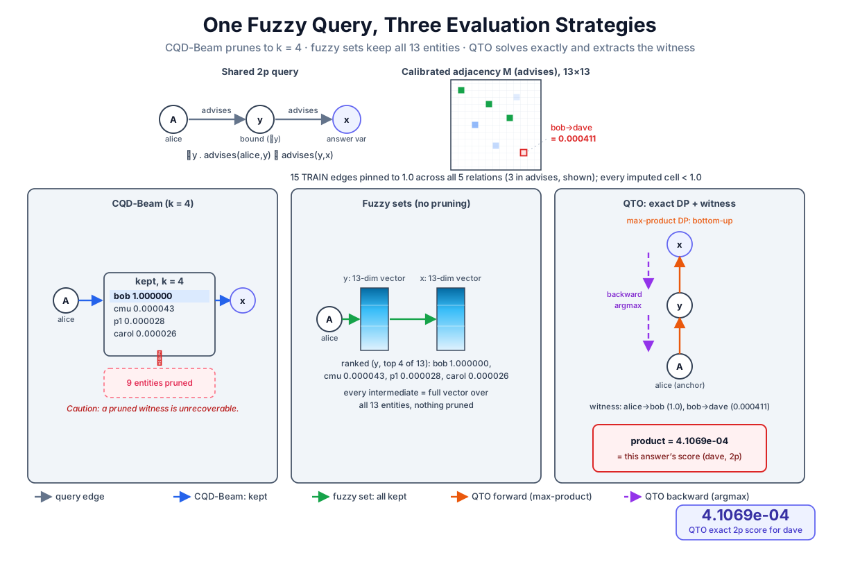One calibrated adjacency matrix, one fuzzy objective, three evaluation strategies: prune to four candidates (CQD-Beam), keep the whole membership vector (the fuzzy-set reading), or solve exactly and extract the witness (QTO). Original diagram by the authors, created with AI assistance.

CQD-Beam: greedy search over concrete entities

CQD's beam variant evaluates the DAG in topological order (children before parents, anchors first) and keeps, at every bound variable, only the top $k$ scoring entities; everything else is zeroed. Here $k$ is the beam width, set to 4 in the committed run; the published system tunes it per dataset, over a grid running from 4 to 256 [1]. The core of the implementation is eleven lines of code plus three comments (cqd.py lines 177–190):

    # Projection chain (sub, (r1, ..., rn)): truncate, hop, repeat.
    if query_dag._is_chain(q):
        assert N not in q[1], "CQD is EPFO-only: no negation atoms"
        v = cqd_beam(q[0], M, k, trace)
        for r in q[1]:
            # Beam: only the top-k bindings of this bound variable survive.
            v = _truncate(v, k)
            if trace is not None:
                beam = [(kg.ENTITIES[i], float(v[i]))
                        for i in np.argsort(-v, kind="stable") if v[i] > 0.0]
                trace.append((r, beam))
            # Atom + ⊤: v'[t] = max_h v[h] · M_r[h,t]  (max-merge of beams).
            v = (v[:, None] * M[kg.R_ID[r]]).max(axis=0)
        return v

The hop line is the 2p objective verbatim: v[:, None] * M[kg.R_ID[r]] forms the $13 \times 13$ array of products $v[h] \cdot M_r[h,t]$, and .max(axis=0) maximizes over the predecessor $h$, merging beams that reach the same tail. The payoff of concrete-entity beams is interpretability: the search state is a short list of named entities with scores, and the committed run prints it for the 2p query:

[2] CQD-Beam trace (k=4, product t-norm) — 2p query:
  q(x) = EXISTS y. advises(alice, y) AND advises(y, x)
  hop 1 (advises ) beam in : alice:1.000000
  hop 2 (advises ) beam in : bob:1.000000, cmu:0.000043, p1:0.000028, carol:0.000026
  final scores (top 3 of 13):
    carol    1.000000   easy answer
    dave     0.000411   HARD answer
    alice    0.000027   non-answer
  dave's score is exactly M[advises][bob, dave] = 0.000411: the pinned
  alice->bob hop costs nothing, the imputed bob->dave hop is the whole price.

Trace the numbers. After hop 1, the beam over the bound variable $y$ holds bob at exactly 1.000000 (the pinned edge alice → bob) and three near-zero stragglers. After hop 2, the hard answer dave scores $1.000000 \times 0.000411 = 0.000411$: the observed hop is free under the product t-norm and the imputed hop is the whole price, which is why dave's final score equals the single matrix entry $M_{\mathrm{advises}}[\mathrm{bob}, \mathrm{dave}]$ (asserted at cqd.py lines 352–353).

Now derive the failure mode the greediness buys. Suppose the true best witness for some answer $x^{\ast}$ is an intermediate $y^{\ast}$ whose score at truncation time ranks below the $k$-th survivor. _truncate (cqd.py lines 135–143) sets $v[y^{\ast}]$ to zero, and every later value is computed only from the surviving vector: the hop reads $\max_h v[h] \cdot M_r[h,t]$, and a zeroed $v[y^{\ast}]$ contributes $0 \cdot M_r[y^{\ast}, t] = 0$ to that max. No later evidence can resurrect a pruned binding, because the recursion never revisits it; the answer $x^{\ast}$ must now ride its best surviving witness, which may score arbitrarily close to zero. Pruning is irreversible, and the error compounds along chains. The committed run does not exhibit a miss: at 13 entities every hard answer's witness tops every k = 4 beam. In eight of the nine cases the witness enters the deciding hop at exactly 1.0 (the anchor's one-hot vector for the 1p and 2i answers, a pinned edge prefix for 2p and pi); for the ip query, whose intersection sits below the final hop, the witness p1 enters the about-hop beam at only 0.000260 (the pinned alice-authored atom times the imputed bob-authored edge) yet still leads its beam, the runner-up scoring 0.000015. So the k = 4 beam and the exact optimum tie rank for rank. Be precise about what exactness guarantees here. Truncation can only lower entries of a nonnegative vector, and every operator above it (product, max) is monotone in its inputs, so the beam's final score for every entity is at most QTO's: the exact scores dominate the beam's entrywise. Score dominance does not by itself force rank dominance: a beam that prunes a non-answer's best witness deflates that rival's score and can hand the hard answer a strictly better rank under the beam than under the exact DP. The QTO ≥ beam ordering on MRR is therefore an empirical fact of this bank, not a theorem, and cqd.py line 381 asserts it as such; here the two tie exactly. At field scale, with thousands of candidates, few pinned prefixes, and $k \ll \lvert V \rvert$ (the beam width far smaller than $\lvert V \rvert$, the number of entities), the cut genuinely bites, at a cost QTO's published comparison quantifies and the committed-table section quotes [2]; CQD's paper also offers a continuous variant that optimizes a relaxed embedding of the bound variables by gradient ascent instead of searching over concrete entities [1].

The fuzzy-set reading: keep everything

The obvious repair is to stop truncating. Keep, at every node of the DAG, the entire membership vector $v \in [0,1]^{13}$: entry $v[e]$ is the fuzzy degree to which entity $e$ belongs to the node's answer set. This is the executor GNN-QE builds its system around [3]: queries decompose into relation projections plus fuzzy-set operations, intersection is the elementwise product, union is the probabilistic sum $1 - \prod_i(1 - v_i)$, negation is the complement $1 - v$, and a projection maps one fuzzy set to its fuzzy image under the relation. In our miniature the fuzzy image goes through the matrix, $v'[t] = \max_h v[h] \cdot M_r[h,t]$, and the reading is literally cqd_beam with the beam widened to all of $V$: at $k = \lvert V \rvert = 13$ the truncation is the identity, nothing is pruned, and the module asserts that the full-width beam agrees with the exact dynamic program on every query in the bank to within $10^{-12}$ (cqd.py lines 326–330):

    # -- QTO ≡ CQD-Beam at full width: the exact DP is the k=|V| beam.
    for t in TYPES:
        for q in QUERY_BANK[t]:
            gap = np.abs(cqd_beam(q, M, k=N_E) - qto_forward(q, M)[0]).max()
            assert gap < 1e-12, f"beam(k=13) diverged from the exact DP: {gap}"

Two consequences follow, one pleasant and one costly. The pleasant one is inspectability: every intermediate state is a ranked list of all entities with degrees, so a debugging session can print what the model believes at any point of the query, exactly as the committed trace printed "final scores (top 3 of 13): carol 1.000000, dave 0.000411, alice 0.000027". Compare BetaE, where an intermediate state is a vector of Beta-distribution parameters that names no entity at all. The costly consequence is that every node now carries a dense $\lvert V \rvert$-sized state; at 13 entities that is 13 floats, at 15,000 entities it is 15,000 per node per query, and the matrix form of projection would need $\lvert V \rvert \times \lvert V \rvert$ per relation. GNN-QE's answer at real scale is to learn the projection: a graph neural network (in the lineage of NBFNet, Neural Bellman-Ford Networks, the same relational message-passing family Volume 3 closed with) takes the current fuzzy set and the relation and produces the next fuzzy set directly, no materialized matrix [3]. Be precise about what that reintroduces. All of GNN-QE's trainable parameters sit in that structure-agnostic projection operator (the fuzzy operations above it are parameter-free algebra, so no structure-specific operator exists to train), but the published system fits the projector end to end on sampled multi-hop queries with their ground-truth answer sets, not on 1-hop links alone; what it deletes is query-structure parameters, not query-level supervision. It is FuzzQE that demonstrates the stronger training-free claim from the embedding side: a query algebra whose conjunction, disjunction, and negation are the operators of a t-norm fuzzy logic (a t-norm, its t-conorm, and the standard complement), satisfying the logical laws by construction, can be trained on plain 1-hop link prediction alone and still answer complex queries competitively [4]. Hold on to this executor: the foundation-models chapter will plug ultra_lite.py's transferable projector into exactly this fuzzy-set loop.

QTO: exact max-product dynamic programming on the query tree

QTO pushes the no-pruning reading to its logical conclusion: if the query DAG is a tree (each bound variable feeds exactly one parent, which holds for all five types in our bank), the fuzzy objective can be maximized exactly, in polynomial time, by dynamic programming, and the maximizing assignment can be recovered afterwards [2]. Both claims deserve their derivations.

Why trees admit exact DP. Two elementary facts about max and products of nonnegative numbers do all the work. First, a nonnegative constant factors out of a max: if $c \ge 0$, then for every $z$ we have $c \cdot f(z) \le c \cdot \max_z f(z)$, so the left side's max is at most the right side; and the bound is attained at the maximizer of $f$, hence

$$\max_z \, c \cdot f(z) \;=\; c \cdot \max_z f(z).$$

Second, a max over disjoint blocks of variables factorizes across a product: if $f \ge 0$ depends only on the block $z_1$ and $g \ge 0$ only on $z_2$, then $f(z_1)\, g(z_2) \le \big(\max_{z_1} f\big)\big(\max_{z_2} g\big)$ for every joint choice, and equality is attained by pairing the two blocks' maximizers, hence

$$\max_{z_1, z_2} \, f(z_1)\, g(z_2) \;=\; \Big(\max_{z_1} f(z_1)\Big) \cdot \Big(\max_{z_2} g(z_2)\Big).$$

Now define, for each node $u$ of the query tree, the vector $T^{\ast}_u[e]$: the maximum, over all assignments of the bound variables strictly below $u$, of the product of the subtree's atom truths, with $u$'s own variable fixed to entity $e$. The tree structure makes this vector computable bottom-up. At an anchor there is nothing below, so $T^{\ast}$ is the one-hot vector. At a projection hop over $r$ from child $c$ to parent $u$, the subtree's atoms are the child subtree's atoms times the new atom $M_r[h, t]$; for a fixed head candidate $h$, the factor $M_r[h,t]$ is a nonnegative constant with respect to the deeper variables, so by the first fact the inner max collapses to $T^{\ast}_c[h]$, and maximizing over the newly bound $h$ gives

$$T^{\ast}_u[t] \;=\; \max_{h \in V} \; T^{\ast}_c[h] \cdot M_r[h, t].$$

At an intersection node, the branches share only the node's own variable, so their bound-variable blocks are disjoint; by the second fact the joint max factorizes into the product of the per-branch maxima, $T^{\ast}_u[e] = \prod_i T^{\ast}_{c_i}[e]$. This disjointness is precisely what a tree guarantees and a general DAG does not: were the same bound variable shared by two branches, the product would couple the blocks and the factorization would be false. The recursion is qto_forward (cqd.py lines 200–237); its chain case memoizes the pre-hop vectors the backward pass will need (lines 222–231). Complexity: one hop costs $\lvert V \rvert^2$ multiply-max operations, so a query with $p$ atoms costs on the order of $p \lvert V \rvert^2$ operations, written $O(p \lvert V \rvert^2)$, against the $\lvert V \rvert^{\text{(number of bound variables)}}$ groundings of brute-force enumeration; the exponential became quadratic because the product distributes over max (exactly the two facts derived above), letting the maxima nest. In the semiring vocabulary of the weighted-model-counting chapter, the DP runs in the max-product semiring, and distributivity is the law that licenses it.

The backward argmax pass. Because each collapse in the forward derivation is an equality attained at a specific maximizer, running the equalities in reverse recovers a witnessing assignment whose atom product is the forward score. Bind the target to an answer $t$, then walk each chain right to left, choosing at every hop the head that attained the max (cqd.py lines 263–272):

    t = t_idx
    hop_atoms: list = []
    for r, v_before in zip(reversed(memo["rels"]), reversed(memo["before"])):
        # Eq. 13:  h = argmax_j T*_before[j] · M_r[j, t]
        h = int(np.argmax(v_before * M[kg.R_ID[r], :, t]))
        hop_atoms.append((kg.ENTITIES[h], r, kg.ENTITIES[t],
                          float(M[kg.R_ID[r], h, t])))
        t = h
    atoms.extend(reversed(hop_atoms))  # report atoms anchor-outward
    qto_backward(memo["child"], M, t, atoms)

At an intersection, every branch inherits the parent's entity and extracts its own chain. The output is a list of grounded atoms, each carrying its matrix value: a faithful proof, in the precise sense that the product of the listed values equals the answer's score exactly, not approximately. The committed run extracts one for the pi query's hard answer:

[3] QTO-lite: exact forward max-product DP + backward argmax proof — pi query:
  q(x) = [EXISTS y. advises(alice, y) AND advises(y, x)] AND advises(bob, x)
  forward T*(x) (top 3 of 13):
    carol    1.0000e+00   easy answer
    dave     1.6867e-07   HARD answer
    alice    3.9755e-11   non-answer
  backward proof for the HARD answer dave (every atom checked against the graph):
    alice --advises--> bob   M = 1.000000   edge-valid: True   TRAIN edge (pinned 1.0)
    bob --advises--> dave   M = 0.000411   edge-valid: True   held-out TEST edge (imputed!)
    bob --advises--> dave   M = 0.000411   edge-valid: True   held-out TEST edge (imputed!)
  product of proof atoms = 1.6867e-07 = T*(dave) — the proof IS the score,
  and it names the held-out edge (bob, advises, dave) it imputed.

Check it edge by edge, as the module does (cqd.py lines 355–366). The chain branch grounds $y$ to bob and rides alice → bob (pinned, 1.0) then bob → dave (imputed, 0.000411); the direct branch grounds its single atom to the same bob → dave edge. Every atom is a real edge of the full graph, and the imputed one is exactly a held-out test edge. One precision note keeps the arithmetic honest: the trace prints each atom rounded to six decimals, and squaring the rounded 0.000411 gives $1.6892 \times 10^{-7}$, not the printed score; at full precision the imputed entry is $4.106935 \times 10^{-4}$, and $1.0 \times (4.106935 \times 10^{-4})^2 = 1.6867 \times 10^{-7}$ reproduces $T^{\ast}(\mathrm{dave})$ to the last printed digit, with the module asserting the full-precision product to within $10^{-15}$ (cqd.py line 361). Notice what the proof also confesses: the same uncertain edge is charged twice, once per branch, so the score is the edge's truth squared. A probabilistic semantics would condition on one world where the edge holds and count it once; the weighted-model-counting chapter built exactly that machinery. The product t-norm is not probability, and the faithful proof is what lets you see the difference in the arithmetic.

The corollary in miniature. QTO's pin is not cosmetic; it carries a guarantee. If an answer is easy (derivable from observed edges alone), its witnessing grounding uses only pinned atoms, so its forward score is a product of exact 1s, which is 1; and since every matrix entry is at most 1, no score exceeds 1, so easy answers sit at the exact top. A non-answer, by contrast, has no grounding on the full graph, so every grounding it offers uses at least one non-observed atom, each capped at $1 - \delta$, bounding its score by $1 - \delta$ strictly below the easy answers. Provable answers therefore rank first, always: the symbolic baseline is never sacrificed for the neural gain. The module states and checks this as the paper's corollary, quantified over the entire bank (cqd.py lines 332–344):

    # -- QTO never misses an EASY answer (Corollary 3.3).  Precisely: for
    #    every query in the 5-type bank, every easy answer's witnessing
    #    grounding uses only pinned-to-1 TRAIN edges, so its forward score is
    #    EXACTLY 1.0; and every non-answer needs at least one non-observed
    #    atom, each capped at 1-δ, so it scores ≤ 1-δ.  Hence every easy
    #    answer ranks strictly ahead of every non-answer: rank 1, never missed.
    for t in TYPES:
        for q in QUERY_BANK[t]:
            T_star, _ = qto_forward(q, M)
            assert all(T_star[kg.E_ID[e]] == 1.0 for e in easy_answers(q)), \
                f"QTO missed an easy answer of a {t} query"
            non = sorted(V - all_answers(q))
            assert max(T_star[kg.E_ID[e]] for e in non) <= 1.0 - DELTA + 1e-12

This is the volume's recurring soundness pattern wearing a new coat: the pinned edges are the symbolic floor, the imputed entries are the neural reach above it, and the theorem says the reach never undermines the floor [2].

The committed table, read honestly

The chapter's verdict is one table: filtered MRR (mean reciprocal rank: for each hard answer, one over its rank among the non-answers, averaged; 1.0 means every hard answer ranked first) over the bank's 9 hard answers, under the Part's filtered protocol (query_dag.py lines 367–408), for five scorers:

[4] hard-answer MRR on the 5-type bank (filtered, query_dag protocol, 9 hard answers)
  model                              1p       2p       2i       pi       ip   pooled
  G_train traversal (symbolic)   0.1484   0.1484   0.1429   0.1484   0.1429   0.1465
  random scorer (seed 0)         0.2250   0.1010   0.1125   0.5625   0.1000   0.2336
  CQD-Beam (k=4)                 0.5500   0.5500   1.0000   1.0000   1.0000   0.8000
  QTO-lite (exact DP)            0.5500   0.5500   1.0000   1.0000   1.0000   0.8000
  G_full oracle (gold ceiling)   1.0000   1.0000   1.0000   1.0000   1.0000   1.0000

Read it row by row, honestly. Symbolic traversal of the training graph pools 0.1465, and not because it is badly built: it scores 0 on every hard answer by definition (hard means "requires a held-out edge"), so its nonzero MRR is pure tie-breaking noise. The random scorer's 0.2336 is the uninformed floor. Both training-free answerers pool 0.8000, and the module asserts the ordering claims rather than eyeballing them: QTO's MRR at least matches the beam's, both beat random by more than 0.2, and QTO beats traversal by the same margin (cqd.py lines 379–387). At this scale exact and greedy tie, and the reason is worth stating exactly: every hard answer's witness tops every k = 4 beam, in eight of the nine cases by entering the deciding hop at exactly 1.0 (an anchor one-hot or a pinned prefix), and in the ip query's case by leading its beam at 0.000260 through the imputed bob-authored edge, so the beam never prunes anything the exact DP needed. Recall from the beam section what exactness actually guarantees: entrywise score dominance, not rank dominance, so the asserted MRR ordering is a verified property of this bank rather than a theorem; the field-scale numbers show what the beam's irreversible pruning costs when it genuinely bites. One reporting convention first: published benchmarks quote MRR multiplied by 100, so a reported 74.0 is 0.740 on this chapter's 0-to-1 scale. On FB15k, a standard benchmark knowledge graph, QTO's exact optimization averages 74.0 across the nine EPFO query types against CQD-Beam's 58.2 [2]: the pruning cost, made measurable. And on FB15k-237, the harder benchmark derived from it, QTO reports 33.5 against BetaE's 20.9 and GNN-QE's 26.8 [2]: the exact optimizer over calibrated 1-hop truths beats every trained query encoder of its era, which is the provocation of this chapter's opening, upgraded from thesis to measurement.

Where did our remaining 0.2 go? Look at the 1p and 2p columns: 0.5500 each, and each column averages exactly two hard answers, so the arithmetic forces one rank of 1 and one rank of 10, since $(1/1 + 1/10)/2 = 0.55$. The rank-1 answer is dave, whose imputed advises edge we watched dominate its rivals. The rank-10 answer is p1 under $\mathrm{authored}(\mathrm{bob}, x)$: the calibrated authored row for bob puts its mass on entities that are not even papers, and the held-out paper lands tenth. Both executors, greedy and exact, inherit that rank identically, because the defect is in the atom layer, not the logic layer; no amount of exact optimization repairs a miscalibrated matrix, and this is the failure the calibration honesty note promised. Note also that intersections helped: 2i, pi, and ip all sit at 1.0000 because the product t-norm punishes candidates that fail any branch, filtering the atom layer's noise.

Last, the compute ledger, because 13 entities hide what 15,000 do not. The neural adjacency here is a dense $5 \times 13 \times 13$ array of 845 floats, precomputed once. At knowledge-graph scale the same object is one $\lvert V \rvert \times \lvert V \rvert$ matrix per relation: with 15,000 entities that is $2.25 \times 10^{8}$ entries per relation before sparsification, and QTO ships only by thresholding near-zero entries into sparse storage [2]. Exactness is bought with quadratic memory; the beam is bought with the risk of pruning the witness; the field currently makes that trade query by query. And the atom scorer underneath all of it is the same 1-hop workhorse throughout: ComplEx, unchanged since Volume 3, whose entire published contribution was a better simple link predictor [5]. "Training-free" is therefore honest only with its qualifier attached: training-free at the query level. The predictor is trained; the calibration is fit to the training graph; what vanished is query-structure training, and that is exactly the piece the previous chapter spent all its parameters on.

The unsolved part

Everything in this chapter hangs from one hook: the calibrated truths. The optimality theorem, the faithful proofs, the corollary about easy answers, all are statements about computing with $M_r$, and the committed table showed one miscalibrated row costing both executors nine ranks that no exactness could buy back. What makes this an open problem rather than an engineering chore is the open world: calibration means matching predicted confidence to the frequency of truth, but the knowledge graph's missing edges are unlabeled, so the frequency of truth is itself unobserved; Volume 5's calibration chapter takes this up as its central question. Negation makes the hook heavier: the complement $1 - x$ maps an overconfident wrong 0.3 to a confident wrong 0.7, so miscalibration is not merely inherited but inverted, and the negation-bearing query types are where fuzzy executors degrade first: on FB15k-237, on the field's multiplied-by-100 scale decoded in the previous section, QTO's negation-type average MRR is 15.5 against its EPFO average of 33.5, and GNN-QE's is 10.2 against 26.8 [2], [3]. And between the beam's speed and the DP's guarantee lies a systems question the field has not closed: an anytime algorithm that widens its beam under a budget and reports, at interruption, a certified bound on how far it can still be from the exact optimum. Nothing in the current toolbox provides that certificate.

Why it matters

This chapter is the volume's cleanest specimen of its title: the logic did not become a loss here, it became the inference engine itself, with a trained model supplying only the atoms. That division of labor is why each piece could be audited separately: the algebra by derivation (the tree DP is exact, proven in four lines of max-product algebra), the atoms by measurement (one bad row, found and named), and the interface by construction (pinned edges guarantee the symbolic floor). The faithful proof is the part Volume 5 will lean on hardest: a system that returns "dave, because alice advises bob and bob advises dave, and I imputed the second edge at 0.000411" has converted a ranking into an auditable claim about specific edges, which is the raw material of trust. The quadratic-memory ledger and the anytime gap are the scale questions, and the reframing itself, competence as inference over a well-calibrated substrate, is the research bet the rest of Part V and the next volume keep testing.

Key terms

• Training-free CLQA (complex logical query answering) — answering multi-hop logical queries using only a pretrained 1-hop link predictor and a fixed fuzzy-logic composition layer, with no training on sampled complex queries; introduced by CQD [1].
• Neural adjacency matrix $M_r$ — per relation $r$, the matrix of calibrated atom truths $M_r[h,t] \in [0,1]$: softmax over candidate tails rescaled by the observed-tail count, capped at $1-\delta$, with observed training edges pinned to exactly 1 [2].
• Calibration — the monotone rescaling of raw predictor scores into $[0,1]$ that makes t-norm composition meaningful; the silent upper bound on every downstream guarantee.
• Fuzzy optimization reading of a query — each candidate answer's truth is the maximum, over assignments of the bound variables, of the product of atom truths; $\wedge$ is the product t-norm, $\exists$ is max, $\vee$ is the probabilistic sum, $\neg$ is the complement $1-x$.
• Beam width $k$ — the number of concrete candidate entities CQD-Beam keeps per bound variable; a pruned witness is unrecoverable, which is the beam's derived failure mode.
• Membership vector (fuzzy set) — the state a no-pruning executor keeps per query node: one degree in $[0,1]$ per entity, inspectable as a ranked list; GNN-QE's representation, with a graph neural network replacing the matrix projection at scale [3].
• Max-product dynamic programming — QTO's exact evaluation on tree-shaped queries: constants factor out of maxima and disjoint variable blocks factorize across products, so bottom-up local steps compute the global optimum in $O(p\lvert V\rvert^2)$.
• Faithful proof (backward argmax) — the witnessing grounding recovered by rerunning each forward max as an argmax; the product of its atom values equals the answer's score exactly, and each atom is checkable against the graph.
• Easy/hard answers — easy answers are derivable from observed edges alone (QTO ranks them first, always, via the pin); hard answers require imputing a held-out edge and are the only ones scored by the filtered-MRR protocol.

Where this leads

Every system in this chapter still trains its atom layer on the one graph it will be asked about: Volume 3's ComplEx knows alice and bob by their rows and would be helpless on a fresh knowledge graph with new entities and new relations. The next chapter, Foundation Models for CLQA, removes that last dependency: ULTRA learns relation representations that transfer to unseen graphs with unseen vocabularies, and UltraQuery mounts exactly this chapter's fuzzy executor on top of the transferable projector, so one pretrained model answers complex queries zero-shot on graphs it has never seen. The logic layer survives unchanged; it is the atom layer's turn to generalize.

---

Companion code: examples/integration/cqd.py implements this entire chapter: the score table and its 845-entry spot-check against Volume 3's ComplEx (lines 77–96 and 307–312), the neural adjacency with cap and pin (lines 99–128), CQD-Beam with its interpretable trace (lines 131–195), the exact tree DP and the backward proof extractor (lines 198–281), and the competency asserts guarding the equivalence, the corollary, the proof's faithfulness, and the table's orderings (lines 326–387). Run python3 examples/integration/cqd.py to reproduce every number in this chapter byte for byte; the run ends with SUMMARY cqd: beam_mrr=0.8000 qto_mrr=0.8000 traversal_mrr=0.1465 random_mrr=0.2336 pinned=15 m_bob_adv_dave=0.000411 proof_atoms=3 proof_valid=True.