Foundation Models for CLQA: LMPNN and UltraQuery

📍 Where we are: Part V · Complex Logical Query Answering — Chapter 18. Fuzzy and Training-Free CLQA removed query training: a fuzzy executor over one calibrated scorer answered every query type with no query-specific parameters. This chapter removes the last dependency, the vocabulary itself.

Every model in this Part so far has shared one silent assumption: the graph it answers queries on is the graph it trained on. Change a single relation name and the machinery collapses, because somewhere inside it sits a learned table with one row per entity or per relation, and a new symbol has no row. A foundation model for reasoning, in the sense the term carries elsewhere in machine learning (one pretrained model applied to many downstream settings without retraining), must answer queries on graphs whose entities and relations it has never seen. That requirement forbids the one design element every prior chapter relied on. This chapter walks the two steps the field took: LMPNN (Logical Message Passing Neural Network), which freezes a pretrained embedding and trains only a light reasoner on top, and ULTRA, which discards symbol-bound parameters entirely by representing each relation through its structural position among the other relations. The companion module ultra_lite.py then runs the claim at toy scale and commits the numbers: a scorer trained only on the academic world answers queries on a disjoint-vocabulary hospital world far above chance, with no gradient update.

The simple version

Imagine a detective who has worked one city for twenty years. Ask her about that city and she is unbeatable, because she knows every name: which family runs which district, who owes whom. Transfer her to a foreign city and the names are gone; her knowledge is worthless. But a different detective never memorized names at all. She learned patterns of roles: the person whom many people report to behaves like a boss, the place where the same people keep appearing behaves like a headquarters, whatever they are called. Drop her in any city and she starts solving cases on day one, because roles are recomputable from scratch wherever she lands. Every embedding model so far is the first detective. This chapter builds the second, and then tests her honestly: train in the academic world, deploy in a hospital world where not one name matches, and measure.

What this chapter covers

• The vocabulary audit: what exactly breaks when each Part-V model meets a new graph (entity rows, relation rows, precomputed adjacency matrices, each named), and the three evaluation regimes (transductive, inductive over entities, inductive over entities and relations) with each prior model placed in the grid; the last cell was empty before this line of work.
• LMPNN, the half step: the query graph whose edges are atoms, the closed-form message derived from a frozen ComplEx-style scorer (a Cauchy–Schwarz argument, worked in full), and the finding that the tiny trained reasoner leans entirely on the frozen table, which is still one graph's vocabulary.
• ULTRA's relation-of-relations graph: the four structural meta-relations (head-to-head, head-to-tail, tail-to-head, tail-to-tail) computed on our own academic graph, a worked Jaccard trace, and the invariance argument that makes "vocabulary-free" a mechanical property rather than a slogan.
• A projector from twelve numbers: source-seeded two-hop propagation with per-hop gates over the structural features, every gradient derived by the chain rule and audited against finite differences at $3.41 \times 10^{-11}$, trained on the academic world only.
• The zero-shot experiment: the hospital world's schema, the frozen-scorer protocol, and the committed three-way table (random 0.2198, zero-shot 0.8333, trained-on-target 0.7500) read carefully, artifact and all.
• UltraQuery in miniature: the previous chapter's fuzzy executor over the zero-shot scorer's calibrated matrices, answering a 2p and a 2i query on the never-seen graph with top-1 answers that are gold hard answers, plus the multi-source subtlety the real system had to fix.
• The Part's verdict: what a reasoning foundation model is (about 177k parameters that transfer) and is not (a model of any domain's content), and why this line of work rediscovers, inside the neural pillar, a property symbolic engines always had.

The vocabulary audit: what every model owns

Run the audit before admiring anything. For each model this Part has built, ask one question: which of its parameters are indexed by a symbol of the training graph? Those parameters are the model's vocabulary, and they are exactly what a new graph invalidates.

model	vocabulary-bound component	what a new graph breaks
GQE, Query2Box, BetaE	one learned row per entity, one per relation	every row: no new entity or relation has one
CQD, LMPNN	a frozen pretrained embedding table (entity rows and relation rows) [1]	the whole table: frozen does not mean portable
GNN-QE (Graph Neural Network Query Executor)	no entity rows (fuzzy sets live on the graph), but learned relation embeddings inside its projector [2]	new relations have no embedding; new entities are fine
QTO	one precomputed $n \times n$ neural adjacency per relation, filled by a transductively trained scorer	both index sets: the matrices are literally shaped by the old vocabulary

Here $n$ is the number of entities in the training graph, so a QTO matrix does not even have a slot for entity $n+1$. The table exposes a hierarchy, and the field names it as three evaluation regimes. In the transductive regime, the test queries range over the same graph the model trained on: same entities, same relations, only the specific edges asked about are new. Everything from GQE (Graph Query Embedding) through QTO (Query Computation Tree Optimization) and LMPNN lives here. In the inductive over entities regime, test-time graphs contain entities never seen in training, but every relation was seen; models in the NBFNet (Neural Bellman-Ford Networks) family reach this cell, because they parameterize relations rather than entities and compute entity representations on the fly by propagation (we meet that backbone formally below). In the inductive over entities and relations regime, nothing at test time was seen in training: new entities, new relations, a new graph. Before ULTRA and its query-answering extension UltraQuery, no single pretrained model reached that cell: link predictors that handle unseen relations did exist (InGram, for one, supplies several of the benchmark graphs ULTRA is evaluated on), but each had to be trained on its own target graph. For complex query answering the cell was genuinely empty; no trained CLQA model could even be applied there, because every prior query-answering architecture required at least a relation vocabulary fixed at training time [3][2].

regime	unseen at test time	Part-V occupants
transductive	nothing but the queried edges	GQE, Query2Box, BetaE, CQD, GNN-QE, QTO, LMPNN
inductive (entities)	entities	NBFNet-style projectors
inductive (entities + relations)	entities and relations	no single pretrained model before ULTRA; no CLQA model at all before UltraQuery [3][2]

The empty cell is not a benchmarking curiosity. It is the difference between a trained artifact and a foundation model: an artifact answers questions about the world it memorized; a foundation model carries a reusable competence into worlds it never saw. The rest of this chapter is the story of how the competence "answer logical queries on a knowledge graph" was separated from the vocabulary it was learned in.

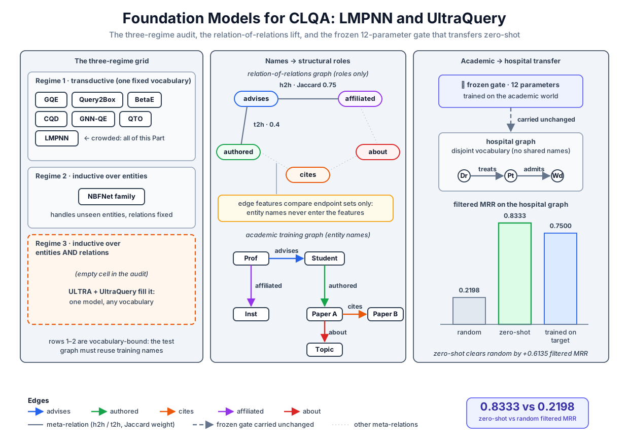The chapter in one picture: the audit's empty cell, the relation-of-relations graph that fills it by replacing names with structural roles, and the committed academic-to-hospital transfer table. Original diagram by the authors, created with AI assistance.

LMPNN: the half step

LMPNN begins from an observation about waste. The transductive CLQA (complex logical query answering) models of the previous chapters each trained a bespoke query encoder from scratch, yet the hardest part of the job, knowing which single edges are plausible, is exactly what an off-the-shelf pretrained knowledge-graph embedding already does well. So LMPNN freezes a pretrained embedding and asks how little machinery must be trained on top of it to answer complex queries [1].

Its object of computation is the query graph: the query's atoms drawn as a labeled graph whose nodes are the constants (anchor entities), the existentially quantified variables, and the single free variable, and whose edges are the atoms themselves, each carrying a relation and possibly a negation flag. The 2i query "who works at St. Luke's and is mentored by Diaz" becomes two edges into one free-variable node. LMPNN runs message passing on this graph: in each round, every atom-edge sends each of its endpoints an estimate of what that endpoint should look like, given the other endpoint's current representation and the frozen scorer.

The crucial move is that these messages are not learned; they are derived from the frozen scorer in closed form. Take the ComplEx-style case, since CQD (Continuous Query Decomposition) already put a frozen ComplEx table in our hands. ComplEx assigns every entity and relation a complex vector of dimension $d$ (the embedding dimension, the number of complex coordinates); write $h, r, t \in \mathbb{C}^d$ for head, relation, and tail, $\bar t_k$ for the complex conjugate of coordinate $t_k$ (flip the sign of its imaginary part), and $\mathrm{Re}(\cdot)$ for the real part. The score of an atom is

$$s(h, r, t) \;=\; \mathrm{Re}\Big(\sum_{k=1}^{d} h_k\, r_k\, \bar t_k\Big).$$

Suppose an atom $r(h, y)$ has a known head and asks about $y$: which tail representation, among all vectors of a fixed length, makes this score largest? Collect the known part into one vector $m = h \odot r$, the elementwise product with coordinates $m_k = h_k r_k$. Write each coordinate in real and imaginary parts, $m_k = a_k + b_k i$ and $t_k = c_k + d_k i$. Multiplying out one term,

$$m_k \bar t_k \;=\; (a_k + b_k i)(c_k - d_k i) \;=\; (a_k c_k + b_k d_k) + i\,(b_k c_k - a_k d_k),$$

so the real part of the sum is $s = \sum_{k=1}^{d} (a_k c_k + b_k d_k)$: exactly the ordinary dot product of the two real vectors of length $2d$ obtained by stacking real parts on imaginary parts. The Cauchy–Schwarz inequality, the same one Volume 1 used to prove steepest descent, then bounds this dot product by the product of the two lengths, with equality precisely when the vectors are parallel. Among all candidate tails of fixed norm, the score is maximized by

$$t^\ast \;\propto\; m \;=\; h \odot r .$$

That is the message: the atom $r(h, y)$ tells node $y$ "the most plausible you, according to the frozen scorer, is the direction $h \odot r$," computed by one elementwise product, no search, no learned parameters. The LMPNN paper tabulates the analogous closed forms for the reverse direction, for negated atoms, and for other frozen scorers [1]. What is trained is deliberately small: one shared multilayer perceptron that aggregates the incoming messages at each node into its next representation, plus two learned vectors used to initialize the nodes that have no frozen row, one for existential variables and one for the free variable. After a few rounds, the free variable's final representation is scored against every entity with the same frozen scorer. The source's ablations report that the division of labor is lopsided: answer quality tracks the quality of the frozen embedding, which is the load-bearing component; the trained network is a light adaptor over it [1].

Score the half step honestly on the audit. Trained parameters indexed by vocabulary: none; the reasoner itself would survive a change of graph. But every message above began with $h \odot r$, and $h$ and $r$ are rows of the frozen table: the vocabulary did not disappear, it moved into the frozen component. Hand LMPNN a hospital graph and it has no row for mentors, no row for adams, and no message to send. The reasoner is portable; the perception of edges is not. The full step has to remove the table itself.

ULTRA: relations described by their position among relations

If a relation may not be represented by a learned row, what is left to represent it by? ULTRA's answer: by its position relative to the other relations of the same graph. Two relations interact structurally whenever their edge sets share endpoints, and there are exactly four ways an ordered pair of relations $(r, r')$ can share them. Write $H(r)$ for the set of entities that appear as heads of $r$-edges and $T(r)$ for the set appearing as tails. The four meta-relations are: head-to-head ($H(r)$ meets $H(r')$: the two relations start from common entities), head-to-tail ($H(r)$ meets $T(r')$), tail-to-head ($T(r)$ meets $H(r')$: where $r$ arrives, $r'$ departs), and tail-to-tail ($T(r)$ meets $T(r')$). Build a new graph whose nodes are the relations and whose edges are these four co-occurrence types: the relation-of-relations graph. A relation's representation is then computed from its neighborhood in this graph, conditioned on the query, by a small network that never touches a name [3].

The academic world makes the construction concrete. The relation advises and the relation affiliated share head entities: bob advises carol and bob is affiliated with mit, so bob belongs to both head sets. That is a head-to-head edge between the two relation-nodes. Likewise advises arrives at carol and affiliated departs from carol, a tail-to-head edge. The companion computes each meta-relation's strength as a Jaccard overlap, the size of the intersection of two sets divided by the size of their union, written $J(A, B) = \lvert A \cap B \rvert / \lvert A \cup B \rvert$; Jaccard is scale-free (it compares proportions, not counts), which is what lets a 13-entity toy graph and a larger one share one parameter vector. For every ordered pair of signed relations (each base relation $r$ plus its inverse inv_r, so that propagation can walk edges backward), the feature row is five numbers: an indicator for "same relation," then the four overlaps (ultra_lite.py lines 168–178):

        def jac(a: set, b: set) -> float:
            return len(a & b) / len(a | b) if a | b else 0.0

        feats = {}
        for r in self.signed:
            for rp in self.signed:
                feats[(r, rp)] = np.array([
                    1.0 if rp == r else 0.0,
                    jac(heads[r], heads[rp]), jac(heads[r], tails[rp]),
                    jac(tails[r], heads[rp]), jac(tails[r], tails[rp])])
        return feats

Work one row by hand, on the real training split. On the 15 academic training edges, $H(\texttt{advises}) = \lbrace \texttt{alice}, \texttt{bob}, \texttt{carol} \rbrace$, $T(\texttt{advises}) = \lbrace \texttt{bob}, \texttt{carol}, \texttt{erin} \rbrace$, $H(\texttt{affiliated}) = \lbrace \texttt{alice}, \texttt{bob}, \texttt{carol}, \texttt{dave} \rbrace$, and $T(\texttt{affiliated}) = \lbrace \texttt{mit}, \texttt{cmu} \rbrace$. Then head-to-head is $J = 3/4 = 0.75$ (three shared heads, four in the union), tail-to-head is $J(\lbrace \texttt{bob}, \texttt{carol}, \texttt{erin} \rbrace, \lbrace \texttt{alice}, \texttt{bob}, \texttt{carol}, \texttt{dave} \rbrace) = 2/5 = 0.4$, and the two people-to-institutions overlaps are $0$ because people and institutions never coincide. The committed run prints exactly this row, next to its hospital counterpart:

    the relation-of-relations features carry the analogy without names:
      f(affiliated | advises)  = [0.   0.75 0.   0.4  0.  ]
      f(worksAt    | mentors)  = [0.   0.75 0.   0.6  0.  ]
      [1 if same relation, then h2h, h2t, t2h, t2t Jaccard overlaps]

Read those two rows slowly, because they are the chapter's mechanism in miniature. Nobody told the model that worksAt plays the role affiliated plays; the near-identical feature rows are that statement, computed from endpoint sets alone. This is what "vocabulary-free" means mechanically: the features are a function of where edges start and end, so two relations with the same structural role receive the same features regardless of what they are called, and a relation renamed to a meaningless token receives identical features. The companion elevates that sentence to an executable assertion (ultra_lite.py lines 542–548): it renames every hospital relation to an opaque token (rel0, rel1, ..., a seeded shuffle), rebuilds the world, recomputes features, and requires the frozen scorer's outputs to agree to $10^{-12}$; the committed run reports a maximum difference of exactly $0.0$. The real system's version of this construction is richer in the same spirit: a graph neural network over the relation-of-relations graph produces, for each query relation, a relative representation of every other relation, and those conditioned representations drive the entity-level scorer [3]. Our miniature keeps the raw feature rows and skips the relation-level network; that honest gap is tallied below.

A projector from twelve numbers

Now the scorer that consumes the features. The design is source-seeded propagation in the style of NBFNet, the backbone the real ULTRA builds on: to score the query $(h, r, ?)$, place unit mass on the source entity $h$ and push it along the graph's edges, letting a learned gate decide, per hop, how much each kind of edge should carry for an $r$-question [4]. Decode the objects first. The number of entities is $n$ (13 in each of our worlds); $x^{(0)} = e_h \in \mathbb{R}^n$ is the one-hot vector with a single $1$ at $h$'s index; for each signed relation $\rho$, $A_\rho$ is the $n \times n$ adjacency matrix with $A_\rho[u, v] = 1$ exactly when the training graph has the edge $(u, \rho, v)$. The hop index is $k \in \lbrace 1, 2 \rbrace$. Each hop owns a gate per signed relation,

$$g_k(\rho \mid r) \;=\; \sigma\!\big(w_k^\top f(\rho \mid r) + b_k\big), \qquad \sigma(z) = \frac{1}{1 + e^{-z}},$$

where $f(\rho \mid r) \in \mathbb{R}^5$ is the structural feature row just built, $w_k \in \mathbb{R}^5$ and $b_k$ are the hop's weights and bias, and $\sigma$ is the logistic squash of Volume 1. The full parameter vector is $\theta = (w_1, b_1, w_2, b_2)$: twelve numbers, and not one of them indexed by a vocabulary item. Gates blend the adjacencies into one gated adjacency per hop, and two hops of propagation produce the score vector (ultra_lite.py lines 253–264):

    g1 = _gates(world, r, theta["w1"], theta["b1"])
    g2 = _gates(world, r, theta["w2"], theta["b2"])
    # G_k = sum_{r'} g_k(r'|r) A_{r'}    (the gated adjacency of hop k)
    G1 = sum(g1[rp][0] * A[rp] for rp in world.signed)
    G2 = sum(g2[rp][0] * A[rp] for rp in world.signed)
    x0 = np.zeros(n); x0[hi] = 1.0
    y = {rp: A[rp].T @ x0 for rp in world.signed}   # y_rho = A_rho^T x0
    x1 = G1.T @ x0
    s = G2.T @ x1                                    # x2: the score vector
    ds_dg1 = {rp: G2.T @ y[rp] for rp in world.signed}
    ds_dg2 = {rp: A[rp].T @ x1 for rp in world.signed}
    return s, ds_dg1, ds_dg2, g1, g2

Unfold the matrix algebra to see what the score is. Entry $a$ of the first hop is $x^{(1)}_a = (G_1^\top x^{(0)})_a = \sum_u G_1[u, a]\, x^{(0)}_u = G_1[h, a] = \sum_{\rho_1} g_1(\rho_1 \mid r)\, A_{\rho_1}[h, a]$, the total gated mass flowing from the source to $a$ in one step. Entry $t$ of the second hop then expands to

$$s_t \;=\; \sum_{a} G_2[a, t]\; x^{(1)}_a \;=\; \sum_{a}\, \sum_{\rho_1, \rho_2} g_1(\rho_1 \mid r)\, g_2(\rho_2 \mid r)\; A_{\rho_1}[h, a]\; A_{\rho_2}[a, t] :$$

a sum over every two-hop path from $h$ to $t$, each path weighted by the product of its two edges' gates. The score is deliberately pure two-hop: the direct edge $(h, r, t)$ is the thing link prediction must impute, so it never scores itself, and during training the positive edge and its inverse are removed from the adjacency before propagation (NBFNet's remove-one-hop discipline, ultra_lite.py lines 242–251), so no example can leak through its own answer. Each score costs two sparse matrix-vector products, linear in the number of signed edges.

The gradients are short enough to derive completely. The score is linear in each gate: from $s = G_2^\top x^{(1)}$ with $G_2 = \sum_\rho g_2(\rho \mid r) A_\rho$, differentiating with respect to one second-hop gate leaves only that gate's term,

$$\frac{\partial s}{\partial g_2(\rho \mid r)} \;=\; A_\rho^\top x^{(1)},$$

and from $x^{(1)} = \sum_\rho g_1(\rho \mid r)\, y_\rho$ with $y_\rho = A_\rho^\top x^{(0)}$, a first-hop gate perturbs $x^{(1)}$ by $y_\rho$, which the whole gated second hop then carries forward:

$$\frac{\partial s}{\partial g_1(\rho \mid r)} \;=\; G_2^\top\, \frac{\partial x^{(1)}}{\partial g_1(\rho \mid r)} \;=\; G_2^\top y_\rho .$$

Those are the two dictionary entries ds_dg1 and ds_dg2 in the excerpt above. Training treats every training edge, in both directions (the tail query $(h, r, ?)$ and the inverse head query $(t, \texttt{inv\_}r, ?)$), as one multiclass example over the filtered candidates of Volume 3's protocol: softmax the candidate scores and minimize $L = -\ln p_{\text{answer}}$. The softmax gradient is the classic cancellation this series has met before (for the sigmoid, in Volume 1 and again in the semantic-loss chapter); here is the softmax version in full. Write $p_e = e^{s_e} / \sum_c e^{s_c}$, where the subscript $e$ names one candidate entity, the index $c$ runs over all filtered candidates in the normalizing sum, and the base $e$ in $e^{s_e}$ is the exponential constant, not the candidate index. Let $y$ be the one-hot answer indicator, so $y_e = 1$ exactly at the answer, $y_e = 0$ elsewhere, and the answer's score can be written $s_{\text{ans}} = \sum_c y_c s_c$. Because $\ln(a/b) = \ln a - \ln b$, the loss expands to $L = -\ln p_{\text{ans}} = -s_{\text{ans}} + \ln \sum_c e^{s_c}$, and differentiating the first term gives $\partial(-s_{\text{ans}})/\partial s_e = -y_e$. Then

$$\frac{\partial L}{\partial s_e} \;=\; \frac{\partial}{\partial s_e}\Big({-s_{\text{ans}}} + \ln \sum_{c} e^{s_c}\Big) \;=\; -y_e + \frac{e^{s_e}}{\sum_c e^{s_c}} \;=\; p_e - y_e .$$

Chain the three links together, using the sigmoid's own derivative $\sigma'(z) = \sigma(z)(1 - \sigma(z)) = g(1-g)$ and $\partial z / \partial w_k = f(\rho \mid r)$:

$$\frac{\partial L}{\partial w_k} \;=\; \sum_{\rho} \underbrace{\Big[\sum_{e} (p_e - y_e)\, \frac{\partial s_e}{\partial g_k(\rho \mid r)}\Big]}_{\text{how much hop-}k\text{'s }\rho\text{ gate mattered}} \; g_k(\rho \mid r)\big(1 - g_k(\rho \mid r)\big)\; f(\rho \mid r),$$

and the same expression without the trailing $f$ for $\partial L / \partial b_k$. The inner training loop is this formula transcribed (ultra_lite.py lines 324–335):

            ex = np.exp(sc - sc.max())
            p = ex / ex.sum()
            loss += -float(np.log(p[ti]))
            dLds = p.copy()
            dLds[ti] -= 1.0                       # dL/ds = p - y
            for rho in world.signed:
                for k, d, g in (("1", d1, g1), ("2", d2, g2)):
                    gv, f = g[rho]
                    # chain rule: dL/dg = (p-y).ds/dg, then sigma' = g(1-g)
                    dLdg = float(dLds @ d[rho][cand]) * gv * (1.0 - gv)
                    grad[f"w{k}"] += dLdg * f
                    grad[f"b{k}"] += dLdg

Full-batch gradient descent on the 30 directional queries of the 15-edge academic split, learning rate $\eta = 0.5$, 300 epochs, produces the committed trace:

[2] training on the academic world only (12 parameters, 300 epochs, 1-vs-all log-loss)
      epoch   mean -ln p(answer)
          1   2.4793
         50   2.4690
        150   2.4591
        300   2.4480
    theta: w1 = [ 0.76  -0.089 -0.585 -0.255  0.577]  b1 = -0.424
           w2 = [ 0.374 -0.409  0.046  0.193  1.333]  b2 = -0.619

[3] gradient audit: all 12 hand partials vs central differences
    max |hand - FD| = 3.41e-11  (< 1e-06)

Two honest readings. First, the loss barely moves, from 2.4793 to 2.4480, and that is structural: the scores are small sums of gated path masses, so the softmax stays close to uniform over the ten to twelve filtered candidates each query ranks (a uniform guess over twelve costs $\ln 12 \approx 2.485$), and twelve parameters could not memorize the answers even if asked. What training changes is the ordering of candidates, which the loss registers faintly and the ranking metrics register decisively. Second, the trained weights are legible at this scale: hop 1's largest weights sit on the same-relation indicator ($0.76$) and the tail-to-tail overlap ($0.577$), and hop 2 leans hardest on tail-to-tail ($1.333$), which reads as "finish an $r$-question along edges that deposit mass where $r$-edges deposit theirs." Every one of the twelve hand-derived partial derivatives is audited against central finite differences on a genuinely two-hop query, agreeing to $3.41 \times 10^{-11}$ (ultra_lite.py lines 503–525). And the distance to the real system is stated, not hidden: real ULTRA runs conditional message passing with non-parametric DistMult messages, sum aggregation, and a learned per-layer transform of the relation representations, over both the relation graph and the entity graph, and it is pretrained on several knowledge graphs at once rather than one 15-edge toy [3][4]. What the miniature preserves is the load-bearing property, vocabulary-freeness, and the shape of the computation.

The zero-shot experiment

Everything so far is architecture; here is the falsifiable core. The companion defines a second world in-module, a hospital: doctors mentor doctors, write reports that reference other reports, work at hospitals, and reports cover specialties (ultra_lite.py lines 102–122):

HOSPITAL_TRAIN: list[tuple[str, str, str]] = [
    ("adams", "mentors", "baker"), ("adams", "mentors", "chen"),
    ("chen", "mentors", "diaz"), ("diaz", "mentors", "evans"),
    ("baker", "wrote", "rep1"), ("chen", "wrote", "rep2"),
    ("evans", "wrote", "rep3"),
    ("rep2", "references", "rep1"), ("rep3", "references", "rep2"),
    ("adams", "worksAt", "mercy"), ("baker", "worksAt", "mercy"),
    ("chen", "worksAt", "stluke"), ("diaz", "worksAt", "stluke"),
    ("rep1", "covers", "cardio"), ("rep2", "covers", "neuro"),
    ("rep3", "covers", "trauma"),
]

# Held out, chosen so each is 2-hop reachable on the train graph (a scorer
# that has learned structural patterns CAN find them; one that has not,
# cannot) — the mentor's hospital, the co-written report, the reference
# closure:
HOSPITAL_TEST: list[tuple[str, str, str]] = [
    ("evans", "worksAt", "stluke"),      # via inv_mentors . worksAt
    ("diaz", "wrote", "rep3"),           # via mentors . wrote
    ("rep3", "references", "rep1"),      # via references . references
]

The schema is deliberately analogous but not isomorphic to the academic world. The role correspondence is plain (mentorship for advising, reports for papers, hospitals for institutions, specialties for topics), and the vocabularies are entirely disjoint: not one entity or relation name is shared. But the shapes differ where it matters. The academic training graph's advising chain is a path, alice to bob to carol to erin; the hospital's mentorship tree branches at its root, adams mentoring both baker and chen. The two academic citations form a chain, while the hospital's three reference edges close a triangle once the held-out rep3 to rep1 edge is included. A model that had merely memorized the academic adjacency pattern would have nothing to match here; only structural regularities of the "roles co-occur this way" kind can carry over. Each of the three held-out edges is two-hop reachable on the hospital training graph, so a scorer that has learned which structural roles to walk can find them, and one that has not, cannot.

The protocol is the definition of zero-shot, executed literally: recompute the structural features on the hospital graph (they are functions of its endpoint sets, nothing else), apply the frozen academic-trained $\theta$, and perform no gradient update of any kind. Evaluation is Volume 3's filtered ranking, hardened: each held-out edge is queried in both directions, known-true competitors are filtered out, and tied scores contribute their expected rank, $\text{rank} = 1 + \#\lbrace e : s(e) \gt s(\text{true}) \rbrace + \tfrac{1}{2}\#\lbrace e : s(e) = s(\text{true}) \rbrace$, where $\#$ counts a set's elements and $e$ ranges over the filtered competitor entities, so a degenerate all-zero scorer lands at chance rather than faking rank 1 (ultra_lite.py lines 348–380). The reported metric is the filtered MRR (mean reciprocal rank: the average, over queries, of one over the answer's rank). Three scorers run under the identical protocol: a frozen random baseline, the zero-shot transfer, and a reference model trained directly on the hospital's own 16 edges. The committed table:

[4] zero-shot link prediction on the hospital world (filtered ranks: tail, head;
    ties at expected rank, so a constant scorer cannot fake rank 1)
      held-out edge                  random     zero-shot  trained-on-target
      (evans, worksAt, stluke)       [3, 2]     [1, 2]     [1, 2]
      (diaz, wrote, rep3)            [12, 11]   [2, 1]     [2, 2]
      (rep3, references, rep1)       [5, 9]     [1, 1]     [1, 1]
      filtered MRR                   0.2198     0.8333     0.7500

Read the three numbers as the finding they are. Random sits at $0.2198$: with 13 entities and heavy filtering, chance is not negligible, which is exactly why the baseline must be run under the same protocol rather than assumed. Zero-shot sits at $0.8333$, with four of the six directional queries ranked first; the module asserts the margin, mrr_zs > mrr_rnd + 0.3, so the transfer claim is load-bearing, not decorative (ultra_lite.py lines 535–536). The gap between those two columns is the chapter's thesis made numerical: twelve numbers fit to one world moved to a world with no shared symbol and still knew where the missing edges were. The third column needs the most care. At this toy scale the trained-on-target reference ($0.7500$) actually falls below the zero-shot transfer, and the module says out loud that this is an artifact: 16 hospital edges are a slightly worse curriculum for these twelve parameters than 15 academic ones, not a harder test. At benchmark scale the published orderings need stating carefully, because one of them shows the same inversion. Against the best reported baselines trained on each specific target graph, zero-shot ULTRA already wins on average, 0.395 versus 0.344 average MRR over the published evaluation suite, so a frozen transfer beating per-graph-trained models is the paper's headline finding, not an anomaly. The comparison that does behave as a skyline is fine-tuning the pretrained model itself, which lifts the average to 0.422, above zero-shot; that fine-tuned-versus-frozen pair, the closest benchmark-scale analogue of our trained-on-target column, is where more training still reliably helps [3]. What is not an artifact, at either scale, is the ordering that matters: zero-shot decisively above chance, on a graph the model never saw.

UltraQuery in miniature: complex queries, zero-shot

One inductive link predictor does not yet answer conjunctive queries. UltraQuery's move is architectural thrift: take the fuzzy-set executor the previous chapter built (fuzzy membership vectors over entities, relation projection as a calibrated one-hop scorer, intersection as a t-norm) and plug the inductive projector into the projection slot [2]. Nothing else changes; the executor was always vocabulary-agnostic, and now the projector is too.

The companion follows the same two steps on the hospital world. First it builds the zero-shot scorer's calibrated matrices: for each signed relation, score every source row, normalize the row into $[0, 1]$ by its own maximum (legitimate because the scores are sums of nonnegative gated path masses), then pin every observed training edge to exactly $1$, the QTO recipe reused from the previous chapter so that provable answers ride for free (ultra_lite.py lines 426–435):

    M = {}
    for r in world.signed:
        rows = []
        for h in world.entities:
            s = score_vec_and_grads(world, h, r, theta)[0]
            m = float(s.max())
            rows.append(s / m if m > 0 else s)
        M[r] = np.vstack(rows)
        M[r][world.A[r] > 0] = 1.0            # pin observed edges
    return M

Then the executor itself, fourteen lines total: an anchor is a one-hot membership vector, projection is the max-product fuzzy image $v'[t] = \max_h v[h]\, M_r[h, t]$ (each candidate tail inherits the best source's membership times that source's calibrated confidence in the hop), and intersection is the elementwise product t-norm (ultra_lite.py lines 443–456). Two committed queries exercise it, each chosen so that its gold answer requires a held-out edge; the gold sets come from query_dag.eval_query, the exact symbolic executor of the CLQA chapters, which is generic over any edge set and so runs on the hospital world unmodified (query_dag.py lines 127–157, called via gold_sets at ultra_lite.py lines 469–474):

Q_2P = ("diaz", ("wrote", "references"))
#   "reports referenced by what diaz wrote" — needs held-out (diaz,wrote,rep3)
Q_2I = (("stluke", ("inv_worksAt",)), ("diaz", ("mentors",)))
#   "who works at stluke AND is mentored by diaz" — needs held-out
#   (evans, worksAt, stluke)

[6] UltraQuery-lite: zero-shot complex queries (fuzzy executor over calibrated matrices)
    2p: diaz -wrote.references->
        easy (train-reachable): {}   hard: ['rep1', 'rep2']
        fuzzy top-3: rep1 0.687, rep2 0.687, rep3 0.571
        top-1 is a gold HARD answer (asserted)
    2i: [stluke -inv_worksAt->] AND [diaz -mentors->]
        easy (train-reachable): {}   hard: ['evans']
        fuzzy top-3: evans 0.715, chen 0.283, adams 0.144
        top-1 is a gold HARD answer (asserted)

Both queries have empty easy sets: symbolic traversal of the hospital training graph returns nothing at all, so every correct answer here is imputation. The 2i case decomposes cleanly under the product t-norm, and it is worth tracing. The candidate chen is certainly at St. Luke's (an observed edge, calibrated membership pinned to $1.0$) but only weakly imputed as diaz's mentee (a two-hop mass calibrating to $0.283$), so its product is $1.0 \times 0.283 = 0.283$. The candidate evans is certainly diaz's mentee (observed, pinned $1.0$) and strongly imputed at St. Luke's ($0.715$), product $0.715$. The conjunction ranks evans first, exactly the gold hard answer, and the module asserts precisely that, for both queries, in two lines (ultra_lite.py lines 563–564):

        assert top[0] in alla, f"{label}: top-1 {top[0]} not a gold answer"
        assert top[0] in hard, f"{label}: top-1 {top[0]} not a HARD answer"

For the 2p query the two gold hard answers rep1 and rep2 tie at the top ($0.687$ each, the printout breaking the tie alphabetically) above every non-answer; note honestly that fuzzy mass also spreads to structurally plausible non-answers like rep3, which is why the assert checks the ranking, not a clean separation. One published subtlety deserves its honest sentence. A projector pretrained for one-hop link prediction always saw a single source with membership $1$; inside a complex query, projection is fed an intermediate fuzzy set with many nonzero entries, a distribution shift the UltraQuery paper had to confront directly, offering two fixes: fine-tune the projector on complex-query data, or keep it frozen and threshold the fuzzy input to sparsify it back toward the pretraining regime [2]. Our miniature sidesteps the shift by construction, because the max-product image applies the calibrated matrix source by source and never propagates a blended fuzzy vector through the network; at full scale, where the projector is itself a propagation conditioned on the source distribution, the shift is real and the fix is part of the system.

What a reasoning foundation model is, and is not

Close the Part by weighing what actually transferred. The published ULTRA model holds about 177k parameters by the paper's count (the released checkpoints tally about 168k), total, for any knowledge graph; a single conventional embedding model for one benchmark graph spends orders of magnitude more than that on its entity table alone, and spends it again for the next graph [3]. Those 177k parameters encode no facts. They encode how evidence flows: which structural role of an edge, relative to the question asked, should carry mass, and how much. That is why the parameters survive a change of world and the embedding tables do not; the tables were the world, the gates are the inference procedure. Two requirements temper the claim. Pretraining needs structural diversity, several graphs of different shapes, or the gates overfit the one topology they saw (the published ablations improve with more pretraining graphs, and our single-graph miniature is below that bar by design [3]). And the whole bet fails where structure carries no signal: relations whose endpoint-set geometry is uninformative, or whose structural role in the new domain differs from every role seen in pretraining, give the gates nothing to grip.

The volume's arc closes here with a symmetry worth saying plainly. query_dag.eval_query, the symbolic executor, answered hospital queries unmodified, because set semantics never depended on names; symbolic engines were always vocabulary-free, and nobody thought to praise them for it. What this line of work achieves is the rediscovery of that property inside the neural pillar, without giving up what the neural pillar was hired for: the committed table's whole point is that the symbolic executor scores $0$ on every hard answer (they require edges it cannot see), while the vocabulary-free neural scorer imputes them at MRR $0.8333$. Generalize over vocabulary and impute missing structure: holding both at once is what earns the word foundation.

The unsolved part

Zero-shot CLQA inherits every upstream fragility this Part catalogued, and inherits them without the safety valve every prior model had: per-graph training that could absorb a mismatch. Calibration is the clearest case. Our pipeline max-normalized score rows into $[0, 1]$ on the new graph, but nothing certifies that a calibrated $0.7$ means the same degree of plausibility in the hospital world as in the academic one, and the product t-norm multiplies those uncertified numbers as if they were commensurable. Negation semantics travel just as badly: the closed-world complement is relative to an entity set the model has no stake in, and a fuzzy complement of a miscalibrated membership vector compounds both errors. Query-bank bias, documented for the transductive benchmarks, does not disappear when the graph changes; it becomes unmeasurable there, because no one has labeled the new world's hard answers. Deeper than all of these sits the assumption the whole construction stands on: that structure carries meaning consistently across domains. It fails exactly where two domains use the same structure differently. In the academic world, the head-to-head overlap between advises and affiliated signals a benign co-location of roles; a graph is easy to imagine in which the same overlap pattern encodes an antagonistic relationship, and the frozen gates cannot tell the two apart, because the feature rows are identical by construction. Whether a model's internal quantities mean what we need them to mean, and how one would ever verify it, is the identifiability question, and it is Volume 5's opening theme, arriving exactly on schedule.

Why it matters

Practically, this chapter is the difference between shipping a reasoner and shipping a reasoner per customer. Every deployment story for CLQA before this line of work began with "first, train an embedding on your graph"; a vocabulary-free projector makes query answering on a fresh knowledge graph a matter of loading 177k frozen parameters and recomputing features, which is why the foundation-model framing is more than branding [3][2]. Conceptually, it settles a question the two pillars have traded all volume: which parts of "reasoning" are knowledge and which are procedure. The committed experiment splits them cleanly, since the knowledge (18 academic facts) demonstrably did not transfer, while the procedure (gate structural roles, propagate, conjoin by t-norm) demonstrably did. Volume 5 will press on both halves: trust (when can a zero-shot answer be believed, given the calibration debts just listed) and scale (whether pretraining across many graphs buys the reliability that per-graph training used to). The honest ledger this chapter carries forward, asserts over vibes, baselines under identical protocols, artifacts named as artifacts, is the method that makes those questions answerable.

Key terms

• Foundation model (for knowledge-graph reasoning) — a single pretrained model applied to new knowledge graphs, entities and relations included, without retraining; requires that no parameter be indexed by a vocabulary item [3].
• Evaluation regimes — transductive (test on the training graph), inductive over entities (new entities, known relations), inductive over entities and relations (nothing shared); no single pretrained model reached the third cell before ULTRA, and no CLQA model at all before UltraQuery.
• LMPNN (Logical Message Passing Neural Network) — CLQA over a frozen pretrained embedding: each query-graph atom sends closed-form messages derived from the frozen scorer, and only a small aggregation network plus two variable-initialization vectors are trained [1].
• Query graph — the query's atoms as a labeled graph over constants, existential variables, and the free variable; the object LMPNN passes messages on.
• Meta-relations (h2h, h2t, t2h, t2t) — the four ways two relations' endpoint sets can overlap (head-to-head, head-to-tail, tail-to-head, tail-to-tail); the edge types of the relation-of-relations graph.
• Relation-of-relations graph — the graph whose nodes are the target graph's relations and whose edges are meta-relation co-occurrences; a relation's representation is its position here, computable on any graph without names [3].
• Jaccard overlap — $J(A, B) = \lvert A \cap B \rvert / \lvert A \cup B \rvert$, the scale-free set similarity the companion uses as meta-relation strength.
• Source-seeded propagation — score $(h, r, ?)$ by placing unit mass at $h$ and pushing it through gated adjacencies, so every tail's score sums its paths' gate products; the NBFNet backbone [4].
• Zero-shot transfer — recompute structural features on the new graph, apply frozen parameters, no gradient updates; here committed as MRR $0.8333$ against a $0.2198$ random floor.
• Relabeling invariance — the executable meaning of vocabulary-free: renaming every relation to an opaque token changes no score (committed maximum difference $0.0$).
• UltraQuery — the inductive projector plugged into the fuzzy-set query executor, answering complex queries zero-shot; at full scale it must handle the multi-source distribution shift by fine-tuning or input thresholding [2].

Where this leads

Part V closed by making the executor portable; the queries themselves were still handed to it as clean symbolic DAGs (directed acyclic graphs). The next Part drops that courtesy: the reasoning problem arrives as English. Soft Reasoners asks whether a language model can be the inference engine, running RuleTaker-style deduction over natural-language rules and facts, and the companion's ruletaker_lite.py puts the same honest instruments (gold proofs, controlled depth, committed accuracy tables) against a reasoner whose vocabulary is, this time, all of language.

---

Companion code: examples/integration/ultra_lite.py implements this entire chapter: the two worlds and their structural features (lines 102–188), the gated two-hop scorer with its hand-derived gradients (lines 211–264), academic-only training (lines 307–342), the hardened filtered-MRR protocol and the relabeling invariance check (lines 348–414), the calibrated matrices and fuzzy executor of UltraQuery-lite (lines 420–474), and the asserts guarding every committed claim, from the finite-difference gradient audit to the zero-shot margin to the gold-hard top-1 answers (lines 496–567). The symbolic gold comes from examples/integration/query_dag.py (eval_query, lines 127–157), unchanged on the hospital world. Run python3 examples/integration/ultra_lite.py to reproduce every number in this chapter byte for byte; the run ends with SUMMARY ultra_lite: mrr_random=0.2198 mrr_zeroshot=0.8333 mrr_trained=0.7500 grad_diff=3.4e-11 invariance=0.0e+00 fuzzy_2p_top1=rep1 fuzzy_2i_top1=evans.