Circuits: SDD, d-DNNF, and Fast Evaluation

📍 Where we are: Part II · Probabilistic Logic and Circuits — Chapter 6. Weighted Model Counting reduced probabilistic inference to a single count and then hit the #P wall; this chapter is the escape route: compile once, count forever.

The previous chapter ended with an honest defeat. Weighted model counting (WMC) is the right currency for probabilistic-logic inference, but computing it on an arbitrary formula is #P-complete, and the brute-force counter paid the full price: every step of four added coins multiplied the enumerated assignments by exactly 16. The defeat, read carefully, contains its own loophole. The hardness result says that no algorithm can count every formula quickly; it says nothing about a formula that has first been rebuilt into a special shape. Knowledge compilation does exactly that: spend a possibly expensive one-time effort translating the formula into a circuit with strong structural guarantees, then answer its menu of supported queries in time polynomial (for the queries this book uses, linear) in the circuit's size [1]. This chapter builds the target shape property by property, proves that each property is precisely what makes one arithmetic operation sound, quotes a working compiler that checks its own guarantees, and ends with the twist that powers the rest of the volume: the same circuit, evaluated under a different algebra, answers a different question.

The simple version

Imagine a tangled heap of extension cords, power strips, and adapters, and you need to know how much current flows out the end. Every time someone asks, you could trace every possible path through the heap from scratch: slow, error-prone, and you pay the full price again for every question. Or you could spend one afternoon rewiring the heap into a clean panel where every junction is labeled and no wire crosses another. The rewiring is real work, sometimes a lot of work. But afterwards, any question (total current, the single strongest path, whether any path is live at all) is answered by one sweep across the panel, reading each junction once. Knowledge compilation is the rewiring; the circuit is the panel; and the different questions are different ways of adding and multiplying at the junctions.

What this chapter covers

• The amortization argument: enumeration pays $2^n$ per query ($n$ the number of probabilistic facts); compilation pays a one-time cost, then answers every downstream query in circuit-size time, with the honest caveat that the circuit itself can be exponential.
• The target language, property by property: negation normal form, then decomposability, determinism, and smoothness, each defined, each motivated by a short proof that it makes one semiring operation correct.
• A real compiler: top-down Shannon expansion on a fixed variable order with a cache, quoted from circuit.py, its OBDD (ordered binary decision diagram) ancestry named honestly.
• Guarantees as checkable code: the three structural properties verified by committed functions, with the PASS lines from the real run.
• One bottom-up pass: the evaluator that turns OR into $+$ and AND into $\times$, matching the brute-force counter to twelve decimals, and the circuit-size-versus-$2^n$ table on the #P-wall family.
• The semiring swap: replacing $(+, \times)$ with $(\max, \times)$ on the same circuit computes the most probable explanation, the first step toward the gradient semiring of the next chapter.
• The compilation map: where d-DNNF (deterministic decomposable negation normal form), SDD (sentential decision diagram), and OBDD sit in the field, and which queries each language supports in polynomial time.

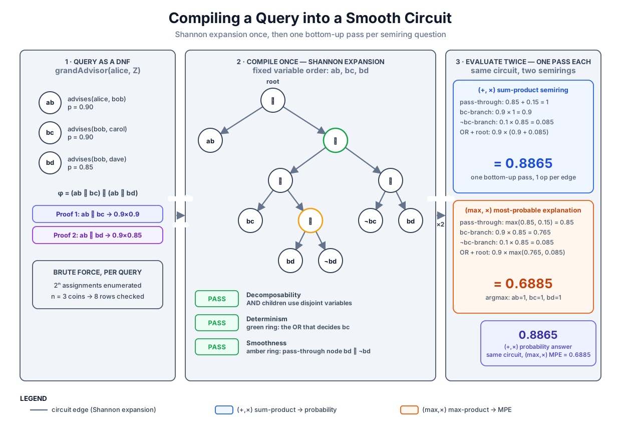Compile once into a smooth d-DNNF circuit, then every query is one bottom-up pass: the semiring chooses the question, the structure guarantees the answer. Original diagram by the authors, created with AI assistance.

Pay once, query forever

Recall the exact cost the previous chapter measured. The brute-force counter wmc.wmc_counted walks all $2^n$ assignments of a formula's $n$ variables, where $n$ is the number of probabilistic facts (the coins) the formula mentions. On the synthetic chain family it enumerated 1,048,576 assignments at $n = 20$, and every query, even a repeat of the same query with new weights, pays the whole bill again.

Compilation reorganizes the ledger. Split the work into two phases:

1. Compile (once per formula): translate the propositional formula $\varphi$ into an equivalent circuit $C$ in a restricted target language. This phase may be expensive; in the worst case the circuit is exponentially large, because if compilation were always cheap and evaluation always linear, we would have a polynomial algorithm for a #P-complete problem, which no one believes exists.
2. Query (as often as you like): answer questions about $\varphi$ by a single bottom-up sweep of $C$, at a cost of one arithmetic operation per circuit edge.

The bet is amortization. A knowledge base changes rarely; queries arrive constantly. If the circuit for the academic world compiles to a few dozen nodes, then re-weighting a coin, conditioning on evidence, or asking for a most probable explanation each cost a linear pass, not a fresh exponential enumeration. The compilation map [1] systematizes this bet across a family of target languages, scoring each on two axes that fight each other: succinctness (how small can circuits in this language be?) and tractable queries (which questions does the language answer in polynomial time?). The more queries a language supports, the more structure its circuits must carry, and the larger they may have to grow. The language this chapter builds sits at a sweet spot of that trade-off, and each of its structural requirements will be earned by a proof, not asserted. One caveat belongs up front: compilation moves the exponential, it does not delete it. The #P wall reappears as a statement about circuit size rather than query time, and the final section returns to exactly where it hides.

The target language, property by property

The target is a circuit: a directed acyclic graph whose leaves are literals or constants and whose internal nodes are labeled AND or OR. We build up its required properties one at a time, and for each one we prove the arithmetic fact that motivates it. Throughout, a literal is a variable $x$ or its negation $\neg x$; an assignment $\omega$ maps every variable to true or false; $\omega \models \varphi$ (read "$\omega$ satisfies $\varphi$", the $\models$ symbol meaning "makes true") says the formula evaluates to true under that assignment. The weight function is the previous chapter's: each variable $x$ carries a probability $p_x$, the literal $x$ has weight $w(x) = p_x$, the literal $\neg x$ has weight $w(\neg x) = 1 - p_x$, and the weight of an assignment is the product of its literal weights. WMC sums assignment weights over the models:

$$\mathrm{WMC}(\varphi, w) \;=\; \sum_{\omega \,\models\, \varphi} \; \prod_{v \in V} w\bigl(v, \omega(v)\bigr),$$

where $V$ is the set of variables $\varphi$ mentions, the subscript $v \in V$ under the product reads "each variable $v$ in the set $V$", and $w(v, \omega(v))$ is $p_v$ if $\omega$ sets $v$ true, $1 - p_v$ otherwise.

Negation normal form

A circuit is in negation normal form (NNF) when negation appears only at the leaves: internal nodes are only AND and OR, and every $\neg$ is glued directly to a variable. Any propositional formula can be rewritten into NNF by pushing negations inward with De Morgan's laws ($\neg(A \wedge B) = \neg A \vee \neg B$ and $\neg(A \vee B) = \neg A \wedge \neg B$) and cancelling double negations, without changing the set of models. NNF alone buys nothing computationally [1]; it is the canvas on which the two load-bearing properties are painted.

Decomposability: what makes × correct

An AND node is decomposable when its children mention pairwise disjoint sets of variables. A circuit is decomposable (a DNNF, decomposable negation normal form) when every AND node is. The point of the property is a counting lemma, and the lemma deserves its full proof because the entire evaluator rests on it.

Lemma (product rule). Let $A$ and $B$ be formulas over disjoint variable sets $V_A$ and $V_B$, meaning $V_A \cap V_B = \emptyset$ (no shared variable). Then

$$\mathrm{WMC}(A \wedge B) \;=\; \mathrm{WMC}(A) \cdot \mathrm{WMC}(B).$$

Proof. An assignment $\omega$ over $V_A \cup V_B$ (their union: the variables belonging to either set) is exactly a pair $(\omega_A, \omega_B)$: its restriction $\omega_A$ to the variables in $V_A$ and its restriction $\omega_B$ to those in $V_B$. Because the sets are disjoint, the pairing loses nothing and duplicates nothing; choosing $\omega$ is the same act as choosing $\omega_A$ and $\omega_B$ independently. Since $A$ mentions only variables in $V_A$, whether $\omega \models A$ depends only on $\omega_A$, and likewise for $B$; therefore $\omega \models A \wedge B$ exactly when $\omega_A \models A$ and $\omega_B \models B$. The weight of $\omega$ splits along the same seam, because a product over $V_A \cup V_B$ is the product of the two sub-products:

$$\prod_{v \in V_A \cup V_B} w\bigl(v, \omega(v)\bigr) \;=\; \underbrace{\prod_{v \in V_A} w\bigl(v, \omega_A(v)\bigr)}_{=\;W(\omega_A)} \;\cdot\; \underbrace{\prod_{v \in V_B} w\bigl(v, \omega_B(v)\bigr)}_{=\;W(\omega_B)}.$$

Now compute the count, replacing the sum over satisfying $\omega$ by the double sum over satisfying pairs, and then factoring the double sum (each term of the first sum multiplies every term of the second, which is precisely what the product of two sums expands to):

$$\mathrm{WMC}(A \wedge B) \;=\; \sum_{\omega_A \models A} \; \sum_{\omega_B \models B} W(\omega_A)\, W(\omega_B) \;=\; \sum_{\omega_A \models A} W(\omega_A) \sum_{\omega_B \models B} W(\omega_B) \;=\; \mathrm{WMC}(A) \cdot \mathrm{WMC}(B). \;\blacksquare$$

(The filled square $\blacksquare$ marks the end of a proof.) Disjointness is not decorative; drop it and the rule fails immediately. Take $A = B = x$ with $p_x = 0.9$. Then $A \wedge B$ is just $x$, so $\mathrm{WMC}(A \wedge B) = 0.9$, but the product $\mathrm{WMC}(A) \cdot \mathrm{WMC}(B) = 0.81$: multiplying treats the two occurrences of $x$ as independent coins when they are one and the same coin. Decomposability is exactly the syntactic condition under which multiplication at an AND node commits no such double-use.

Determinism: what makes + correct

An OR node is deterministic when its children are pairwise logically disjoint: no assignment satisfies two of them. A decomposable circuit whose ORs are all deterministic is in deterministic decomposable negation normal form (d-DNNF) [1]. The motivating lemma is the mirror image of the product rule.

Lemma (sum rule). Let $A$ and $B$ be formulas over a common variable set such that $A \wedge B$ is unsatisfiable. Then

$$\mathrm{WMC}(A \vee B) \;=\; \mathrm{WMC}(A) + \mathrm{WMC}(B).$$

Proof. Write $\mathrm{Mod}(\varphi)$ for the set of assignments satisfying $\varphi$. Always $\mathrm{Mod}(A \vee B) = \mathrm{Mod}(A) \cup \mathrm{Mod}(B)$, by the truth table of OR. Because $A \wedge B$ is unsatisfiable, no assignment lies in both sets: the union is disjoint. A sum over a disjoint union splits into the two partial sums, each term landing in exactly one:

$$\mathrm{WMC}(A \vee B) \;=\; \sum_{\omega \in \mathrm{Mod}(A) \,\cup\, \mathrm{Mod}(B)} W(\omega) \;=\; \sum_{\omega \in \mathrm{Mod}(A)} W(\omega) \;+\; \sum_{\omega \in \mathrm{Mod}(B)} W(\omega) \;=\; \mathrm{WMC}(A) + \mathrm{WMC}(B). \;\blacksquare$$

Without determinism the correct identity is inclusion–exclusion, $\mathrm{WMC}(A \vee B) = \mathrm{WMC}(A) + \mathrm{WMC}(B) - \mathrm{WMC}(A \wedge B)$, and naively adding overcounts every doubly-satisfying assignment. This is the trap the distribution-semantics chapter exposed as the disjoint-sum problem: grandAdvisor(alice, Z) has two proofs sharing the coin advises(alice, bob), and adding their probabilities gave the absurd "probability" $0.81 + 0.765 = 1.575$, when the true answer is $0.8865$. Determinism is that trap's structural cure. Instead of correcting the overlap after the fact with inclusion–exclusion terms (whose number explodes with the number of proofs), the compiler rebuilds the formula so overlap can never occur: every OR in the output is, by construction, a choice between "$x$ is true here" and "$x$ is false here", and no assignment can take both branches.

Smoothness: the bookkeeping property

One more property makes circuits pleasant rather than correct-for-counting. An OR node is smooth when all its children mention exactly the same set of variables. Why care? Consider an OR whose left child mentions $\{x\}$ and whose right child mentions $\{x, y\}$. The left child's count is silently a count over assignments to $x$ alone; the right child's is over assignments to both. Adding them mixes two different sample spaces. For probability weights the mixture happens to be harmless, and it is worth seeing exactly why: a variable $y$ missing from a child can be freely true or false, so its contribution to that child's share of the full-space count is the factor

$$w(y) + w(\neg y) \;=\; p_y + (1 - p_y) \;=\; 1,$$

and multiplying by 1 changes nothing. The repair that makes this reasoning structural is equally simple: for each missing variable $y$, multiply the deficient child by the pass-through node $\mathrm{pt}(y) = (y \vee \neg y)$. The pass-through is itself a deterministic OR (its children decide $y$ oppositely) and a decomposable AND-mate (it introduces only the missing $y$), so the repair preserves d-DNNF; and under $(+, \times)$ it evaluates to exactly the factor 1 just computed, so the count is unchanged. A smooth d-DNNF is the full target language. The reason smoothness earns its keep is that other semirings are not so forgiving: $\max(p_y, 1 - p_y)$ is not 1 unless $p_y$ is exactly $\tfrac12$, and the demo below shows an un-smoothed circuit silently corrupting a most-probable-explanation query while leaving the probability query untouched.

The compiler: Shannon expansion with a cache

How does one actually produce a circuit with these properties? The companion's compiler, circuit.py, uses the oldest trick in the book, the Shannon expansion: any formula $\varphi$ splits on any variable $x$ as

$$\varphi \;=\; (x \wedge \varphi|_{x=1}) \;\vee\; (\neg x \wedge \varphi|_{x=0}),$$

where $\varphi|_{x=1}$ (the cofactor, also called the residual) is $\varphi$ with $x$ replaced by true and simplified, and $\varphi|_{x=0}$ replaces it by false. Read the identity as a case split: every assignment sets $x$ one way or the other, the left disjunct collects exactly the models with $x$ true, the right those with $x$ false. Both required properties fall out of the shape of the split. The OR is deterministic because its children force $x$ to opposite values, so no assignment satisfies both. Each AND is decomposable because the cofactor no longer mentions $x$ (it was substituted away), so the literal child and the residual child have disjoint variable sets. Recursing on the residuals, always branching on the first variable of a fixed order that the residual still mentions, and caching each residual so that repeated subformulas compile to one shared node, yields a d-DNNF circuit. Here is the core, verbatim (circuit.py lines 266–282):

    def build(residual: tuple) -> int:
        if residual == ():                 # no terms: unsatisfiable, φ = ⊥
            return b.add(("F",))
        if residual == (frozenset(),):     # empty term: satisfied, φ = ⊤
            return b.add(("T",))
        if residual in cache:
            return cache[residual]
        # Branch variable: the order-first variable the residual mentions.
        x = order[min(rank[v] for t in residual for v, _ in t)]
        # φ = (x ∧ φ|x=1) ∨ (¬x ∧ φ|x=0); builder simplification prunes the
        # ⊥ branch (AND with ⊥ = ⊥, dropped from the OR) and ⊤ conjuncts.
        hi = b.AND([b.lit(x, True), build(_cofactor(residual, x, True))])
        lo = b.AND([b.lit(x, False), build(_cofactor(residual, x, False))])
        cache[residual] = b.OR([hi, lo])
        return cache[residual]

    return _compact(b.nodes, build(dnf), order, dnf)

Honesty about ancestry: a fixed variable order plus a cache of residuals is precisely the recipe for an ordered binary decision diagram (OBDD), read here as a circuit; the toy is an OBDD compiler wearing d-DNNF clothes. Industrial compilers are considerably smarter. The sentential decision diagram (SDD) generalizes the linear variable order to a binary vtree over the variables and supports combining two compiled circuits in polynomial time, while remaining canonical [2]; compilers from conjunctive normal form (CNF, an AND of OR-clauses) to d-DNNF, such as those behind ProbLog2 [3] and the ACE system, extract circuits from the trace of an exhaustive DPLL (Davis–Putnam–Logemann–Loveland)-style backtracking search with component caching and clause learning [4]. What the toy shares with all of them is the contract, not the engineering: the output language and the guarantees that come with it. Raw Shannon output has one flaw left, already announced: it is not smooth (a residual that becomes ⊤ mentions no variables at all), so compile() (circuit.py lines 322–332) runs the smooth() repair pass after expansion, inserting pass-through nodes wherever an OR's children disagree on scope (circuit.py lines 307–317):

        else:  # "O": pad every child up to the union scope of all children
            union: frozenset = frozenset()
            for c in rest[0]:
                union |= circuit.scope[c]
            kids = []
            for c in rest[0]:
                missing = sorted(union - circuit.scope[c], key=repr)
                inserted += len(missing)
                pts = [b.OR([b.lit(v, True), b.lit(v, False)]) for v in missing]
                kids.append(b.AND([new[c]] + pts))
            new.append(b.OR(kids))

Trace the compiler by hand on the running example, because the whole chapter's machinery fits in it. The query grandAdvisor(alice, Z) compiles (in wmc.py) to the two-proof disjunctive normal form (DNF, an OR of AND-terms) $\varphi = (ab \wedge bc) \vee (ab \wedge bd)$, where $ab$ abbreviates the coin advises(alice, bob) with $p_{ab} = 0.9$, $bc$ is advises(bob, carol) with $p_{bc} = 0.9$, and $bd$ is advises(bob, dave) with $p_{bd} = 0.85$. The sorted order branches on $ab$ first. The cofactor $\varphi|_{ab=0}$ kills both terms (each demands $ab$), leaving the empty DNF ⊥, so the whole $\neg ab$ branch is pruned. The cofactor $\varphi|_{ab=1}$ is $bc \vee bd$, which branches on $bc$: the true branch's residual is ⊤ (the term $\{bc\}$ is fully satisfied), the false branch leaves $bd$. The raw circuit is therefore

$$ab \;\wedge\; \bigl(\, bc \;\vee\; (\neg bc \wedge bd) \,\bigr),$$

7 nodes and 6 edges, and its inner OR is un-smooth: the left child mentions $\{bc\}$, the right $\{bc, bd\}$. The repair pads the left child to $bc \wedge (bd \vee \neg bd)$, one pass-through inserted, giving the smooth circuit of 10 nodes and 10 edges. Those sizes are not hand-waved; they are the committed compile table:

[1] compile: top-down expansion, then the smoothness repair
      query                        vars terms |  raw nodes edges | smooth nodes edges  +pt
      grandAdvisor(alice, carol)      2     1 |          3     2 |           3     2    0
      citesTransitively(p3, p1)       2     1 |          3     2 |           3     2    0
      colleague(carol, erin)          1     1 |          1     0 |           1     0    0
      grandAdvisor(alice, Z)          3     2 |          7     6 |          10    10    1

The contract, checked as code

A guarantee you cannot check is a rumor. The properties of the last section are object properties of a finished circuit, decidable by inspection, and circuit.py inspects them on every run rather than trusting the compiler's construction argument. Decomposability is a set computation: for every AND node, the children's variable scopes must be pairwise disjoint, which holds exactly when the size of their union equals the sum of their sizes (circuit.py lines 379–392):

def check_decomposable(circuit: Circuit) -> int:
    """Decomposability: for every AND node the children's scopes are
    pairwise DISJOINT (sizes add up exactly).  Returns the number of AND
    nodes checked; raises AssertionError on any violation."""
    n_and = 0
    for i, (kind, *rest) in enumerate(circuit.nodes):
        if kind != "A":
            continue
        n_and += 1
        # |∪ scopes| = Σ |scope| ⇔ pairwise disjoint.
        assert len(circuit.scope[i]) == sum(len(circuit.scope[c])
                                            for c in rest[0]), (
            f"AND node {i} has overlapping child scopes")
    return n_and

Determinism is checked twice, once structurally (every OR is a binary decision whose children force one variable to opposite values, circuit.py lines 395–419) and once semantically, by the bluntest possible instrument: enumerate all $2^n$ assignments over the circuit's $n$ variables, evaluate every node under the Boolean semiring, and demand that no assignment ever satisfies two children of one OR (circuit.py lines 422–438). The enumeration check is affordable only at toy scale (the code refuses beyond $n = 10$), which is exactly why it is valuable here: at this scale, "the ORs are deterministic" is not an argument but an exhaustively verified fact. Smoothness is checked by comparing child scopes per OR (circuit.py lines 441–452). The committed run stamps all four:

[2] the d-DNNF contract, checked as code (structure, never assumed)
      decomposability : 5 AND nodes across 4 circuits, child scopes pairwise disjoint            PASS
      determinism     : 2 OR nodes, each a decision x vs ¬x (structural)                         PASS
      determinism     : exhaustive, all 4+4+2+8 = 18 assignments, no OR children overlap         PASS
      smoothness      : raw circuits have 1 un-smooth OR; repaired with pt(v) = (v ∨ ¬v): 0 remain PASS

One pass, twelve decimals

Now the payoff. On a smooth d-DNNF, weighted model counting is a single bottom-up sweep of the node list: a literal leaf reads its weight, an AND multiplies its children's values (sound by the product rule, because the compiler guaranteed disjoint scopes), an OR adds its children's values (sound by the sum rule, because the compiler guaranteed disjoint models). The evaluator is one short loop, and it counts its own work: exactly one arithmetic operation per circuit edge (circuit.py lines 344–365):

    for i, (kind, *rest) in enumerate(circuit.nodes):
        if kind == "F":
            vals[i] = sr.zero
        elif kind == "T":
            vals[i] = sr.one
        elif kind == "L":
            var, sign = rest
            vals[i] = weights[var][0] if sign else weights[var][1]
        elif kind == "A":
            # AND → ⊗ over children (decomposability makes this sound).
            v = sr.one
            for c in rest[0]:
                v = sr.times(v, vals[c])
                ops += 1
            vals[i] = v
        else:
            # OR → ⊕ over children (determinism makes this sound).
            v = sr.zero
            for c in rest[0]:
                v = sr.plus(v, vals[c])
                ops += 1
            vals[i] = v

Run it by hand on the smooth grandAdvisor(alice, Z) circuit, leaves upward. The pass-through evaluates to $0.85 + 0.15 = 1$. The padded left branch is $0.9 \times 1 = 0.9$; the right branch is $0.1 \times 0.85 = 0.085$; the OR adds them, $0.9 + 0.085 = 0.985$; the root AND multiplies in the shared coin, $0.9 \times 0.985 = 0.8865$. That is the exact value the previous chapter obtained by enumerating all $2^3$ assignments, and the committed run confirms all four academic queries at twelve decimals, with the operation count equal to the edge count every time:

[3] ONE bottom-up (+, ×) pass == wmc.py's 2^n brute force, to 1e-12
      query                        circuit WMC      wmc.py brute     |diff|   ops = edges
      grandAdvisor(alice, carol)   0.810000000000   0.810000000000   0.0e+00     2 = 2
      citesTransitively(p3, p1)    0.720000000000   0.720000000000   0.0e+00     2 = 2
      colleague(carol, erin)       0.550000000000   0.550000000000   0.0e+00     0 = 0
      grandAdvisor(alice, Z)       0.886500000000   0.886500000000   1.1e-16    10 = 10

The academic circuits are tiny, so the amortization argument needs the scaling family to bite. The previous chapter's #P-wall family ($k$ independent two-coin chains, $n = 2k$ variables, closed form $1 - 0.44^k$) compiles to circuits whose node count grows linearly in $n$: the chains share no variables, so each chain adds a constant-size gadget, and the residual cache never re-expands a suffix it has seen. The committed table puts the two price tags side by side:

[6] the escape from the #P wall (wmc.py's chain family, compiled)
      n   k  2^n assignments   nodes  edges  ops    circuit WMC        1 − 0.44^k       |diff|
       8   4              256      41     64   64    0.962519040000   0.962519040000   0.0e+00
      12   6            4,096      65    114  114    0.992743686144   0.992743686144   0.0e+00
      16   8           65,536      89    172  172    0.998595177637   0.998595177637   0.0e+00
      20  10        1,048,576     113    238  238    0.999728026391   0.999728026391   0.0e+00
      growth per +4 coins: nodes +24 (LINEAR); edge increments [50, 58, 66]
      (quadratic — the smoothing price); brute-force assignments: exactly 16× per step
      at n = 20: 238 semiring ops vs 1,048,576 assignments — 4,405× fewer

Read the gap aloud. Brute force multiplies its work by exactly 16 at every step, by construction; the compiled circuit adds 24 nodes per step, a constant. At $n = 20$ the circuit answers in 238 semiring operations what enumeration answers in 1,048,576 weighted assignments, a factor of 4,405, and the two agree to machine precision against the closed form. (The edge count grows quadratically rather than linearly; that is the smoothing repair's price, since later chains must be padded with pass-throughs for earlier chains' variables, and the run asserts both growth laws as constant first and second differences, circuit.py lines 644–648.) This linear-versus-exponential separation on a family whose raw enumeration is provably $2^n$ is the entire business case for compilation-based exact inference [4].

The semiring swap: same circuit, new question

Look back at the evaluator excerpt. Nothing in it says "probability". It folds OR children with sr.plus starting from sr.zero and AND children with sr.times starting from sr.one, where sr is a commutative semiring: a set equipped with two operations $\oplus$ and $\otimes$ and two distinguished elements $\bar 0$ and $\bar 1$, such that $\oplus$ is associative and commutative with neutral element $\bar 0$, $\otimes$ is associative and commutative with neutral element $\bar 1$, $\otimes$ distributes over $\oplus$, and $\bar 0$ absorbs under $\otimes$ (anything times $\bar 0$ is $\bar 0$). The two proofs of this chapter used only these laws plus the disjointness facts the structure guarantees; nothing used subtraction or division. So the same compiled circuit answers a different question whenever a different semiring's $\oplus$ and $\otimes$ are plugged into the same pass. This is algebraic model counting [5], and it is the abstraction the rest of Part II rides.

The first swap is $(\max, \times)$. Define the most probable explanation (MPE) of $\varphi$ as the satisfying assignment of maximum weight, and its value as that maximum:

$$\mathrm{MPE}(\varphi, w) \;=\; \max_{\omega \,\models\, \varphi} \; \prod_{v \in V} w\bigl(v, \omega(v)\bigr).$$

The sum rule becomes a max rule: over a union of model sets, the maximum is the larger of the two partial maxima, $\max(\mathrm{MPE}(A), \mathrm{MPE}(B))$, and here determinism is not even needed, because unlike $+$, the $\max$ of overlapping sets counts nothing twice ($\max$ is idempotent: $\max(a, a) = a$). The product rule survives verbatim, because a maximum over independent choices factors: the best pair $(\omega_A, \omega_B)$ is the best $\omega_A$ paired with the best $\omega_B$, so $\max_{(\omega_A,\omega_B)} W(\omega_A) W(\omega_B) = \bigl(\max_{\omega_A} W(\omega_A)\bigr)\bigl(\max_{\omega_B} W(\omega_B)\bigr)$, using that all weights are non-negative. But now smoothness is load-bearing. A variable missing from an OR child contributed the harmless factor $p + (1-p) = 1$ under addition; under $\max$ the pass-through contributes $\max(p, 1 - p)$, the price of choosing the free variable's better value, and omitting that factor means the un-smoothed circuit prices the variable at 1, an overestimate whenever $p \ne \tfrac12$. The committed run exhibits exactly this failure and its repair on the running query, where the raw circuit's ⊤ branch never mentions advises(bob, dave):

[4] why smoothness matters: SAME circuit, (max, ×) semiring
      grandAdvisor(alice, Z): the raw circuit's ⊤ branch never mentions
      advises(bob, dave), so (max, ×) pays factor 1 instead of max(0.85, 0.15):
        un-smooth (max, ×) = 0.810000   OVERESTIMATE
        smooth    (max, ×) = 0.688500   = enumerated max (0.90 · 0.90 · 0.85)
      (+, ×) never notices: un-smooth WMC = 0.886500 is already exact,
      because a skipped variable contributes p + (1 − p) = 1 anyway

Check the smooth value by hand: the pass-through now contributes $\max(0.85, 0.15) = 0.85$, the padded left branch is $0.9 \times 0.85 = 0.765$, the right branch $0.1 \times 0.85 = 0.085$, the OR takes $\max(0.765, 0.085) = 0.765$, and the root gives $0.9 \times 0.765 = 0.6885$, the weight of the all-true assignment $ab \wedge bc \wedge bd$. The maximizing assignment itself is recovered by a downward argmax pass: starting at the root, descend through every child of an AND, but at an OR descend only into a child whose value equals the node's value (such a child exists because the node's $\max$ is attained by some child), and read the chosen literals off the leaves (circuit.py lines 456–480). Smoothness is again what makes the decoded assignment total: every variable under an OR occurs in every branch, so no variable escapes the descent unassigned, and the code asserts totality explicitly (circuit.py lines 478–479). The committed decode, verified against exhaustive enumeration:

      grandAdvisor(alice, Z)       MPE = 0.688500
        argmax: advises(alice, bob)=1, advises(bob, carol)=1, advises(bob, dave)=1

Two semirings, one circuit, and the table has an announced third row:

task	$\oplus$	$\otimes$	$\bar 0$	$\bar 1$	needs determinism?	needs smoothness?	reads off
probability (WMC)	$+$	$\times$	$0$	$1$	yes (sums double-count)	no ($p + (1-p) = 1$)	$P(q)$
most probable explanation	$\max$	$\times$	$0$	$1$	no ($\max$ is idempotent)	yes ($\max(p, 1-p) \ne 1$)	best proof world
gradient (next chapter)	pairwise $+$	product rule on pairs	$(0,0)$	$(1,0)$	yes	yes	$\bigl(P(q),\ \partial P(q)/\partial p\bigr)$

The third row is the reason this chapter exists inside a volume about differentiable logic. If the value carried through the circuit is not a number but a pair (a probability and its derivative with respect to a fact's weight), and $\oplus$ and $\otimes$ are defined so that the second component obeys the sum and product rules of calculus, then the same bottom-up pass computes exact gradients of the query probability with respect to every probabilistic fact. That is the gradient semiring, and it is how a neural network will be trained through exact logical inference in the next chapter.

Where compilation lives in the field

The toy compiler drops into a mature ecosystem. ProbLog2 grounds a probabilistic logic program to a weighted Boolean formula, compiles it with a d-DNNF compiler or to an SDD, and evaluates semirings on the result [3]; the compile-then-evaluate pipeline is the standard architecture of exact probabilistic-logic inference [4]. The compilation map organizes the possible target languages by containment: OBDD circuits are a special case of SDD and SDDs are d-DNNF [2]; d-DNNF is DNNF, DNNF is NNF, and each step up the chain is at least as succinct (every circuit of the lower language already belongs to the higher one, so the smallest higher-language circuit can only be smaller or equal) while supporting fewer polynomial-time queries [1]. A condensed view of the trade-off, for the queries this book uses:

language	satisfiability	weighted counting $(+, \times)$	MPE $(\max, \times)$	model enumeration
NNF	intractable	intractable	intractable	intractable
DNNF (decomposable)	polytime	intractable	polytime (smoothed)	polytime
d-DNNF (+ determinism)	polytime	polytime	polytime (smoothed)	polytime
SDD	polytime	polytime	polytime (smoothed)	polytime
OBDD	polytime	polytime	polytime (smoothed)	polytime

("Intractable" means: not in polynomial time unless P equals NP, or unless the polynomial hierarchy collapses, per the map's conditional results [1]; the MPE column follows from the semiring argument above, which needs decomposability and smoothness but tolerates non-determinism [5].) Why ever prefer a weaker language? Succinctness: demanding more polytime queries costs circuit size, and the map proves separations between neighboring rows. SDD earns its industrial role by adding what no unrestricted d-DNNF has, a canonical form (fixing the vtree fixes the circuit) and a polytime apply operation that conjoins or disjoins two compiled SDDs directly, which is what incremental systems need when the formula grows clause by clause [2]. The same decomposable-product, smooth-sum structure, with determinism as an optional extra property and with weights generalized from literal probabilities to learned distributions, is the modern definition of a probabilistic circuit, the umbrella under which sum-product networks and their relatives now live [6]; the machinery this chapter built for logic is, almost symbol for symbol, the machinery of tractable probabilistic modeling.

The unsolved part

The exponential did not die; it moved into the compiler, and its new address is the variable order. The chain family compiled to linear-size circuits partly because sorted order happened to keep each chain's two coins adjacent, so every residual was small and the cache kept hitting. Order matters enormously in general: for OBDD-style compilation there are classic formula families (the multiplexer-like functions are the textbook case) whose circuits are linear under one order and exponential under another, so the choice of order alone can swing the compile from trivial to hopeless. And choosing well is itself hard: even improving a given OBDD's order is NP-complete [7], so real compilers fall back on heuristics (min-fill orderings, hypergraph partitioning for vtrees, dynamic reordering) with no optimality guarantee [2]. The toy is honest about its position on this ladder: it uses the sorted variable order, never searches, and never reorders (circuit.py lines 45–49 state this out loud). The semantics of this chapter, meaning both correctness proofs and both semiring evaluations, are airtight; what is unsolved is the quality of compilation, the gap between the circuit you get and the smallest circuit that exists. The #P wall stands. Compilation does not breach it; it relocates the toll booth to compile time, where a knowledge base that changes rarely can afford to pay it once.

Why it matters

This chapter is the load-bearing floor of everything the volume builds next. DeepProbLog trains neural networks through exact probabilistic inference; that is affordable only because the inference is a differentiable circuit pass, not an enumeration. Semantic loss (Part III) compiles a logical constraint into a circuit once, then backpropagates through it at every training step; the amortization argument is literally its training loop. Scallop's provenance semirings and the gradient semiring of the next chapter are new rows of this chapter's semiring table, evaluated by the same one-pass evaluator. Further ahead, Volume 5's trust story leans on the fact that circuit evaluation is exact: when a probability estimate comes from a d-DNNF pass, agreement with the semantics to $10^{-12}$ is a checkable property, not a hope, which is precisely the kind of guarantee the reasoning frontier is short of. The two pillars meet here with unusual symmetry: the symbolic pillar contributes the formula and the proofs of soundness, the neural pillar will contribute the weights, and the circuit is the room where they transact.

Key terms

• Knowledge compilation: translate a formula once into a target language with structural guarantees, then answer the language's supported queries in time polynomial (for this chapter's queries, linear) in the compiled circuit's size; systematized by the compilation map's succinctness-versus-queries trade-off [1].
• NNF (negation normal form): internal nodes only AND and OR, negation confined to the leaves; the canvas language, with no tractability of its own.
• Decomposability: every AND's children mention pairwise disjoint variable sets; exactly the condition under which $\mathrm{WMC}(A \wedge B) = \mathrm{WMC}(A)\,\mathrm{WMC}(B)$.
• Determinism: every OR's children are pairwise logically disjoint; exactly the condition under which $\mathrm{WMC}(A \vee B) = \mathrm{WMC}(A) + \mathrm{WMC}(B)$ needs no inclusion–exclusion correction; the structural cure for the disjoint-sum problem.
• Smoothness: every OR's children mention the same variable set, restorable by pass-through nodes $\mathrm{pt}(v) = (v \vee \neg v)$; a no-op under $(+, \times)$ since $p + (1-p) = 1$, but load-bearing under $(\max, \times)$, where the pass-through prices a free variable at $\max(p, 1-p)$.
• d-DNNF (deterministic decomposable negation normal form): the target language combining all of the above; counting, MPE, and enumeration each run in one bottom-up pass.
• Shannon expansion: $\varphi = (x \wedge \varphi|_{x=1}) \vee (\neg x \wedge \varphi|_{x=0})$; applied recursively on a fixed order with a residual cache it yields an OBDD-style d-DNNF, deterministic and decomposable by construction.
• SDD (sentential decision diagram): the industrial target generalizing OBDD's variable order to a vtree; canonical, with a polytime apply operation [2].
• Commutative semiring: the algebra $(\oplus, \otimes, \bar 0, \bar 1)$ the evaluator is generic over; $(+, \times)$ reads off probability, $(\max, \times)$ the MPE, and the gradient semiring (next chapter) the derivative, all from one circuit [5].
• MPE (most probable explanation): the maximum-weight satisfying assignment; computed by the $(\max, \times)$ pass and decoded by descending, at each OR, into a child attaining the node's value.
• Probabilistic circuit: the umbrella term for computation graphs with decomposable products and smooth (optionally deterministic) sums, covering compiled logical circuits and learned tractable models alike [6].

Where this leads

The semiring table ended with an announcement: a row whose carried value is a pair, probability together with its derivative. The next chapter, DeepProbLog: Neural Predicates and the Gradient Semiring, cashes that announcement in. A neural network's softmax output becomes the probability label on a literal leaf; the circuit pass computes the query probability exactly; the gradient semiring runs the same pass on (value, derivative) pairs, handing the network a true gradient of a logical query's probability with respect to its own weights. Logic stops being a post-processor bolted onto a network and becomes a differentiable layer inside it, and the proofs of this chapter are what make that layer's forward pass exact rather than approximate.

---

Companion code: examples/integration/circuit.py implements this entire chapter: the semiring objects (lines 71–90), the Shannon-expansion compiler with its residual cache (lines 247–282), the smoothness repair (lines 285–319), the one-pass evaluator counting one operation per edge (lines 336–374), the three structural checks (lines 379–452), MPE with argmax decoding (lines 456–480), the brute-force oracle (lines 485–510), and the run that asserts every number quoted here (lines 519–661), consuming the certified DNFs of examples/integration/wmc.py via export_for_circuit() (wmc.py lines 240–252). Run python3 examples/integration/circuit.py to reproduce every table byte for byte; the run ends with SUMMARY circuit: queries=4 max|circuit-brute|=1.1e-16 unsmooth_mpe=0.8100 true_mpe=0.6885 wall_n=20 ops=238 assignments=1048576 max|circuit-closed|=0.0e+00.