The Work-Depth Trilemma

📍 Where we are: Part IV · Scale and Systems — Chapter 11. GPU Reasoning made each wave of the completion fixpoint cheap by turning it into matrix algebra; this chapter counts the one thing batching cannot touch, the number of waves that must run in order.

The previous chapter ended with a fixpoint whose every round was one batched tensor pass, and a fair question hanging: if a round is now a single matrix operation, is the reasoner fast? That question has two different answers because cost has two different axes. Work is the total number of operations a computation performs, summed over everything, everywhere. Depth is the length of the longest chain of operations in which each one needs the previous one's result, so no amount of hardware can overlap them. Parallel machines shrink running time toward the depth; they never push it below the depth. This chapter measures reasoning on both axes with the companion module work_depth.py, and finds the frontier is not one line but three: plain reachability can trade a mountain of extra work for exponentially less depth, the EL completion core cannot make that trade at all (and the theory says why), and between the two sits the engineering dial this volume will keep turning, a kernel cut off after a fixed number of rounds, which stays perfectly sound at every budget and pays only in recall. A third axis, memory, is counted only implicitly here and returns at the end as the honest reason the chapter's title says trilemma rather than trade-off.

The simple version

Imagine catering a wedding with as many helpers as you like. Addressing five hundred invitations parallelizes perfectly: five hundred helpers, one minute, done. Reducing a stock does not: it must simmer, then reduce, then be tasted, each stage needing the previous stage's result, and ninety-nine extra cooks do not shorten a ninety-minute simmer by one second. That simmer time is depth. The total labor bill, every minute worked by every helper, is work. Sometimes you can buy depth down with work: a pressure cooker finishes the stock in a third of the time by spending far more energy per minute. And sometimes chemistry refuses the deal: no gadget lets the tasting happen before the reduction it tastes. Reasoning has exactly these three situations, and this chapter counts, on committed code, which rules of inference are invitations, which are pressure-cookable stocks, and which are stubborn chemistry.

What this chapter covers

• Work and depth from scratch: both quantities defined by counting on the smallest possible example (summing a list of numbers), why depth lower-bounds running time on any number of processors, and the honest converse, that work is the bill someone always pays.
• Reachability priced both ways: the linear wave kernel against repeated squaring of the reachability matrix, both quoted from the committed code, both asserted equal to an independent reference, with the counted depth/work table at chain lengths 8, 64, and 512 and the classical theorem (transitive closure is in NC²) stated precisely.
• The core that refuses the trade: a five-rung alternation ladder on which label derivations and edge derivations need each other in strict alternation, so the fixpoint takes 11 waves over a role graph of diameter 1, and a constant-round squaring pipeline provably undershoots on one gadget and unsoundly overshoots on another.
• The complexity wall, imported with discipline: EL subsumption and Datalog closure are PTIME-complete, and PTIME-complete problems admit no polylogarithmic-depth, polynomial-work algorithm unless NC = P; the theorem is cited, the conjecture's status stated, and the toy is presented as the mechanism, never the proof.
• The truncation law: cutting the wave kernel off after L rounds is sound at every L (an exact subset assert, derived from monotonicity) and complete exactly at L = D; the committed recall-versus-L curve, and why truncation's error direction is the opposite of an embedding's.
• The three-tier scaling law: constant-depth rewriting, logarithmic-depth squaring, linear-depth waves, assembled into one table with each row's fragment, depth, work, and evidence, plus the reading discipline that scalability belongs to the fragment before it belongs to the system.
• Where the dial reappears: fixed-depth networks, chain-of-thought decoding, and the SATORI kernel's fixed-L unrolling, each named as this chapter's law in different clothes.

Work and depth, defined by counting

Take the smallest computation with any structure at all: summing a list of $n$ numbers $a_1, a_2, \ldots, a_n$, where $n$ is the length of the list and $a_i$ is the number in position $i$. The obvious loop computes $((a_1 + a_2) + a_3) + \cdots$: it performs $n - 1$ additions, and every addition waits for the previous one's result, so both its total operation count and its longest dependent chain are $n - 1$. Now reorganize the same additions into a balanced tree: pair the numbers up and add each pair simultaneously, leaving about half as many values; pair those up; repeat. Every addition still consumes two values and produces one, and the computation starts with $n$ values and ends with $1$, so exactly $n - 1$ additions happen no matter how they are scheduled. But the number of rounds changes completely: each round at least halves the count of surviving values, so after $t$ rounds at most $\lceil n / 2^t \rceil$ values remain (the ceiling brackets $\lceil \cdot \rceil$ round up to the next integer), and one value remains as soon as $2^t \ge n$, that is, after $t = \lceil \log_2 n \rceil$ rounds, where $\log_2 n$ is the power to which $2$ must be raised to give $n$. The two schedules define the two quantities of this chapter [1]:

• Work $W$: the total number of operations executed, here $n - 1$ under both schedules.
• Depth $D$: the length of the longest chain of operations in which each needs its predecessor's output, here $n - 1$ for the loop and $\lceil \log_2 n \rceil$ for the tree.

The pair matters because of a machine-independence fact. On an idealized parallel machine with $p$ processors (the PRAM, parallel random-access machine, the standard abstraction in which every processor can read and write a shared memory each step [1]), the running time $T_p$ obeys two lower bounds at once: $T_p \ge W / p$, because $p$ processors execute at most $p$ operations per step and all $W$ operations must happen; and $T_p \ge D$, because the operations on the longest dependent chain must execute one after another regardless of how many processors sit idle. A matching upper bound, Brent's scheduling bound, says $T_p \le W/p + D$: greedy scheduling achieves both floors up to their sum [1]. Read the two floors as the chapter's two morals. Depth is the part of the cost no purchase order can remove: it bounds time on any number of processors. Work is the part someone always pays: every counted operation costs energy and hardware occupancy, so an algorithm that halves depth by squaring work is not free, it has moved the cost from the clock to the electricity bill.

One bookkeeping convention before anything is counted, restated from the module's counting-convention block so the numbers below are auditable (work_depth.py, lines 75–82): the counted operations are the boolean-semiring operations of the closure computation itself. A dense $n \times n$ boolean matrix product counts $n^2 (2n - 1)$ operations, because each of the $n^2$ output cells performs $n$ AND-probes and $n - 1$ OR-reductions. The sparse wave kernel counts one operation per join probe and one per successful merge of a genuinely new pair. Fixpoint-detection comparisons (matrix equality, emptiness of a frontier) are counted in neither kernel, so the comparison is apples to apples.

Reachability, closed two ways

The first testbed is the most reasoning-shaped problem that parallelizes well: reflexive-transitive closure, deciding for every pair of nodes $(i, k)$ in a directed graph whether some path leads from $i$ to $k$. In the running example this is exactly atomic subsumption. The nf1 slice of Volume 2's normalized academic TBox (the terminological box, the ontology's axiom set), every axiom of the shape $A \sqsubseteq B$ between concept names (read: every $A$ is a $B$; the relation $\sqsubseteq$ is called subsumption), is a directed graph (the module imports it from ontology.py through el_completion.normalize, never retyping it; work_depth.py, lines 184–192), and the derived subsumptions $A \sqsubseteq^{*} B$ are precisely the reachable pairs. A longest chain is $\mathsf{Dean} \sqsubseteq \mathsf{Professor} \sqsubseteq \mathsf{Researcher} \sqsubseteq \mathsf{Person}$ (two chains through $\mathsf{TenuredStudent}$ tie it at three edges). Alongside it the module closes a family of worst-case chains $v_0 \to v_1 \to \cdots \to v_{n-1}$ at $n = 8, 64, 512$. In this section and its reachability table, $D$ denotes the graph's diameter, the longest finite shortest-path distance between any two nodes, computed by an independent breadth-first search that touches neither counted kernel (work_depth.py, lines 364–384), and both kernels are asserted equal to a third, plain depth-first-search reference (lines 405–406), so neither is ever graded against the other alone.

The wave kernel: D − 1 rounds of little work

The first kernel is the semi-naive closure, the same frontier discipline that Volume 1's forward-chainer and the previous chapter's delta trick used: keep the closure found so far, and each round join only the newest pairs (the frontier $\Delta$) against the base edges $M$, so that every pair is derived exactly once (work_depth.py, lines 108–139):

    closure: set[tuple[str, str]] = {(u, u) for u in nodes} | set(edges)
    delta = set(closure)
    depth = 0
    ops = 0
    while delta:
        new: set[tuple[str, str]] = set()
        for i, j in delta:
            for k in out.get(j, ()):
                ops += 1                       # one ∧-probe of the join Δ ⋈ M
                if (i, k) not in closure and (i, k) not in new:
                    ops += 1                   # one ∨-merge of a new pair
                    new.add((i, k))
        if not new:
            break
        closure |= new
        delta = new
        depth += 1
    return closure, depth, ops

Its depth is exactly $D - 1$ rounds, and this can be derived rather than observed. Write $R_t$ for the closure held after $t$ productive rounds. The invariant is that $R_t$ contains exactly the pairs at distance at most $t + 1$. Base case: $R_0$ is initialized to $I \vee M$, the identity pairs (distance $0$) together with the base edges (distance $1$), so the invariant holds at $t = 0$. Inductive step: for $t \ge 1$ the frontier $\Delta_t$ holds exactly the pairs whose shortest distance is $t + 1$ (they were new at round $t$; at $t = 0$ the frontier additionally holds the identity pairs, but joining $(i, i)$ with an edge $(i, k)$ only reproduces a base edge already in $R_0$, so those extra members add nothing new). The round joins each $(i, j) \in \Delta_t$ with each base edge $(j, k) \in M$, extending shortest paths of length $t + 1$ by one edge to paths of length $t + 2$; every path so produced that is genuinely new has length exactly $t + 2$, and conversely any pair first reachable at distance $t + 2$ has such a decomposition (its shortest path's last edge is some $(j, k) \in M$, and the prefix has length exactly $t+1$), so the round adds exactly the distance-$(t{+}2)$ pairs. New pairs therefore exist precisely while $t + 2 \le D$, giving $D - 1$ productive rounds, which is what the module asserts on every graph (line 408).

The counted work is startlingly small, and on the chain it has a closed form. Each closure pair $(i, j)$ enters the frontier exactly once, and contributes one probe per out-edge of $j$; on the chain every node has one out-edge except the last. The closure of the $n$-chain has $\sum_{i=0}^{n-1} (n - i)$ pairs, where the summation symbol $\sum$ adds up the term $n - i$ once for every $i$ from $0$ to $n - 1$; the sum equals $n(n+1)/2$ (node $v_i$ reaches itself and everything after it, contributing $n - i$ pairs). Probes: the pairs whose second coordinate has an out-edge number $n(n+1)/2 - n = n(n-1)/2$. Merges: the pairs not already present in $R_0$ number $n(n+1)/2 - (2n - 1) = (n-1)(n-2)/2$. Factoring $(n-1)$ out of both terms:

$$\frac{n(n-1)}{2} + \frac{(n-1)(n-2)}{2} \;=\; \frac{(n-1)\big(n + (n-2)\big)}{2} \;=\; (n-1)^2 .$$

For $n = 512$ that predicts $511^2 = 261{,}121$ counted operations, and the committed table below shows exactly that number. The wave kernel does essentially no wasted work; its cost is the depth, $510$ strictly ordered rounds.

Repeated squaring: ⌈log₂ D⌉ rounds of much work

The second kernel attacks the depth directly. Form the boolean matrix $A_0 = I \vee M$ (entry $(i,k)$ is true when $i = k$ or $(i,k)$ is a base edge) and repeatedly square it under the boolean matrix product $\odot$, in which multiplication is AND and addition is OR (work_depth.py, lines 142–174):

    A = np.eye(n, dtype=bool) | M
    productive = 0
    executed = 0
    ops = 0
    while True:
        A2 = bmm(A, A)
        executed += 1
        # n² cells × (n ∧-probes + (n−1) ∨-reductions) per dense product.
        ops += n * n * (2 * n - 1)
        if np.array_equal(A2, A):
            break
        A = A2
        productive += 1

The invariant now doubles instead of incrementing: $A_t$ holds exactly the pairs joined by a path of length at most $2^t$. Base case: $A_0 = I \vee M$ covers lengths $0$ and $1$, that is, at most $2^0$. Inductive step: the product's definition is $A_{t+1}[i,k] = \bigvee_j A_t[i,j] \wedge A_t[j,k]$, where $\bigvee_j$ ORs over every intermediate node $j$; any path of length $\ell \le 2^{t+1}$ can be split at the node reached after $\min(\ell, 2^t)$ steps into two halves of length at most $2^t$ each, and conversely two such halves concatenate to a path of length at most $2^{t+1}$, so the invariant carries. The fixpoint is reached once $2^t \ge D$, after exactly $\lceil \log_2 D \rceil$ productive squarings, plus one final squaring whose only job is to certify that nothing changed; the module asserts both counts on every graph (lines 411–413). One subtlety earns its own committed demonstration: the identity must be ORed in before squaring. Bare $M^{2^t}$ holds only walks of length exactly $2^t$, so on an acyclic graph it forgets every shorter path and collapses; writing $\lvert M \rvert$ for the number of true entries of $M$ (a count, not a determinant), on the 7-edge chain the module verifies $\lvert M \rvert = 7$, $\lvert M^2 \rvert = 6$, $\lvert M^4 \rvert = 4$, $\lvert M^8 \rvert = 0$, the zero matrix (lines 443–449).

The price is density. Every executed squaring is a full dense product costing $n^2(2n-1)$ counted operations whether or not the matrix is sparse. At $n = 512$: $512^2 = 262{,}144$ cells, $2 \cdot 512 - 1 = 1023$ operations per cell, so $268{,}173{,}312$ operations per squaring, and $10$ executed squarings give $2{,}681{,}733{,}120$. Here is the committed table, quoted from the module's real output (run python3 examples/frontier/work_depth.py):

[1] the reachability slice, closed two ways (both == DFS reference)
                             linear semi-naive        (I ∨ M) squaring
  graph                n    D    waves          ops   sq(+1)            ops     work ratio
  chain n=8              8    7        6           49      3+1          3,840        78.4x
  chain n=64            64   63       62        3,969      6+1      3,641,344       917.4x
  chain n=512          512  511      510      261,121      9+1  2,681,733,120    10,270.1x
  academic ⊑-preorder    6    3        2           19      2+1          1,188        62.5x

Read the two directions of the trade off one row. At $n = 512$ the depth falls from $510$ ordered rounds to $9{+}1$, matching $\lceil \log_2 511 \rceil = 9$, while the counted work rises from $261{,}121$ to $2{,}681{,}733{,}120$, a factor of $10{,}270$. Both directions are guarded, not just displayed: the module asserts the productive squaring count equals $\lceil \log_2 D \rceil$ and asserts the squaring work strictly exceeds the linear work on every instance, the assert comments calling it what it is, log depth bought with work (lines 411–419). The academic preorder row lands the same law on the running example: the $\mathsf{Dean}$-to-$\mathsf{Person}$ chain gives $D = 3$, two waves or $2{+}1$ squarings, $19$ against $1{,}188$ counted operations. And because this slice is a fragment of the real calculus, the module closes the loop on soundness: every derived pair $A \sqsubseteq^{*} B$ is asserted to sit inside full classification's saturated labels, $B \in S(A)$, checked against the raw completion state because the full TBox proves $\mathsf{TenuredStudent} \sqsubseteq \bot$ ($\bot$ is the bottom concept, the concept with no members, so the class is unsatisfiable) and the polished report hides unsatisfiable concepts (lines 424–433).

The theory behind the squaring column is a classical theorem, and the house rule for imported theory applies. NC (Nick's Class) is the family of problems solvable by uniform families of boolean circuits of polynomial size and polylogarithmic depth; $\text{NC}^k$ restricts the depth to $O(\log^k n)$, meaning depth grows at most as a constant times the $k$-th power of $\log n$. Decoded: NC is exactly "massively parallelizable in principle", polynomial work organized into an extremely shallow dependency structure. The theorem: the reflexive-transitive closure of a directed graph on $n$ vertices is computable in $\text{NC}^2$, by circuits of polynomial size and $O(\log^2 n)$ depth [1]. The two logarithms are visible in the kernel just quoted: $\lceil \log_2 D \rceil$ squaring stages, each stage a boolean matrix product whose $\bigvee_j$ over $n$ terms is itself a balanced OR-tree of depth $\lceil \log_2 n \rceil$. The proof of the theorem, including the circuit-uniformity conditions, is beyond this volume; what the companion demonstrates instead is the mechanism and its counted price, the schedule of $\lceil \log_2 D \rceil$ dense products and the $10{,}270$-fold work bill at $n = 512$.

The core refuses the trade

So the academic hierarchy squares. Why can the full completion calculus not be squared the same way? Because its depth is not reachability depth. The EL completion of Volume 2 maintains two kinds of state, concept labels $S(X)$ (the derived superclasses of $X$) and role edges $(X, Y) \in R(r)$, and its rules read one kind to write the other. The module isolates the mechanism in a $k$-rung alternation ladder, a TBox already in Volume 2 normal form (work_depth.py, lines 196–212):

    axioms: list[tuple] = [("nf1", "A0", "M0")]
    for i in range(k):
        axioms.append(("nf3", f"M{i}", "r", f"B{i}"))
        axioms.append(("nf4", "r", f"B{i}", f"M{i + 1}"))

In description-logic (DL) syntax: $A_0 \sqsubseteq M_0$; then for each rung $i$, $M_i \sqsubseteq \exists r.B_i$ (read: every $M_i$ has an $r$-successor in $B_i$, so the label $M_i$ emits a role edge) and $\exists r.B_i \sqsubseteq M_{i+1}$ (anything with an $r$-successor in $B_i$ is an $M_{i+1}$, so that edge yields the next label). The saturation kernel is the lockstep wave version of the completion rules, each wave firing all of CR1, CR3, CR4 on the frozen previous state (work_depth.py, lines 245–291): CR1 propagates atomic subsumptions into labels, CR3 turns a label $A \in S(X)$ with $A \sqsubseteq \exists r.B$ into an edge $(X, B) \in R(r)$, and CR4 turns an edge $(X, Y) \in R(r)$ with $B \in S(Y)$ and $\exists r.B \sqsubseteq C$ into the label $C \in S(X)$. Trace the dependency at concept $A_0$: the label $M_{i+1} \in S(A_0)$ can only be produced by CR4 reading the edge $(A_0, B_i)$, and that edge can only be produced by CR3 reading the label $M_i \in S(A_0)$. Each new label costs one CR3 wave plus one CR4 wave, the seed label costs one CR1 wave, so the deepest fact $M_k \in S(A_0)$ arrives at wave $2k + 1$, and the module asserts exactly that, along with exact fact-for-fact equality against Volume 2's el_completion.complete oracle (lines 458–460).

Now the punchline that separates this depth from the previous section's. The role graph this ladder derives is bipartite: every edge runs from a subject ($A_0$ or some $M_i$) to some $B_j$, and no edge ever leaves a $B_j$, so no two-edge path exists at all. Its proper transitive closure adds zero pairs, and the module asserts as much (lines 463–464). Committed output:

[3] the non-squarable core: the k=5 alternation ladder
    (A0 ⊑ M0;  Mi ⊑ ∃r.Bi;  ∃r.Bi ⊑ M(i+1)) — wave t+1's rule
    firing needs wave t's LABEL, interleaved with brand-new edges
    lockstep fixpoint == el_completion oracle: 68 facts in 11 waves (2k+1)
    the derived role graph is bipartite: transitive closure adds 0
    pairs — diameter 1, yet depth 11: the depth is NOT reachability

A role graph of diameter $1$ forced $11$ ordered waves. The depth lives in the alternation between fact kinds, exactly the structure repeated squaring cannot see, because squaring accelerates paths within one relation and the ladder never grows a path longer than one edge.

The constant-round strawman: undershoot and overshoot

Perhaps squaring just needs to be applied more cleverly? The module builds the cleverest schedule that still has constant depth, the strawman naive_squared_pipeline (lines 304–355): (1) close the atomic-subsumption graph by squaring (exact: that is the reachability slice), (2) one fully parallel CR3 pass, (3) transitively close each role matrix $R(r)$ by squaring, (4) one fully parallel CR4 pass, (5) close the subsumption graph again. Five rounds, a constant independent of the instance, each round polylog-depth: this is what any constant-round schedule built from squaring primitives must look like. (A schedule allowed polylogarithmically many alternation rounds would crack this $k = 5$ ladder, but fails the same way on any ladder whose rung count exceeds its round budget; the claim that no polylog-depth schedule of any shape works is the conditional theorem of the next section, not something one gadget can exhibit.) It fails in both possible directions, and the module asserts each failure exactly.

On the ladder it undershoots. One CR3 pass followed by one CR4 pass advances each dependency chain by exactly one label-edge pair, and the fixpoint needs $k$ such alternations. Count what the five rounds miss: at $A_0$, the labels $M_2, \ldots, M_k$ and the edges $(A_0, B_1), \ldots, (A_0, B_{k-1})$, which is $2(k-1)$ facts; at each $M_i$, the labels $M_{i+2}, \ldots, M_k$ and the edges $(M_i, B_{i+1}), \ldots, (M_i, B_{k-1})$, which is $2(k - 1 - i)$ facts, summing over $i = 0, \ldots, k-1$ to $2 \cdot k(k-1)/2$. The total is

$$2(k-1) + 2\,\frac{k(k-1)}{2} \;=\; 2\left((k-1) + \frac{k(k-1)}{2}\right),$$

which at $k = 5$ is $2(4 + 10) = 28$. The module asserts the strawman's output is a strict subset of the truth, asserts the missing count is exactly this formula, and asserts the deepest label $A_0 \sqsubseteq M_5$ is among the missing (lines 468–472): $40$ facts derived of the true $68$.

On a second gadget it overshoots, which is worse. The two-hop TBox is $X \sqsubseteq \exists r.Y$, $Y \sqsubseteq \exists r.Z$, $\exists r.Z \sqsubseteq C$ (lines 215–221). The true completion derives $C \in S(Y)$ only: CR4 looks through one role edge, and $X \sqsubseteq \exists r.\exists r.Z$ does not entail $X \sqsubseteq \exists r.Z$, because EL roles do not compose without an explicit chain axiom. The semantics makes this concrete with a three-element countermodel: take domain $\{x, y, z\}$ with $r = \{(x,y), (y,z)\}$, $X = \{x\}$, $Y = \{y\}$, $Z = \{z\}$, $C = \{y\}$. All three axioms hold ($x$ has an $r$-successor in $Y$; $y$ has one in $Z$; the only element with an $r$-successor in $Z$ is $y$, and $y \in C$), yet $x \notin C$, so $X \sqsubseteq C$ is not entailed. Step (3) of the strawman, treating $R(r)$ as a reachability relation, invents the edge $(X, Z)$, and step (4) then derives $C \in S(X)$. The module asserts the overshoot is exactly these two facts and nothing else (lines 480–484):

    two-hop gadget (X ⊑ ∃r.Y, Y ⊑ ∃r.Z, ∃r.Z ⊑ C): squaring R(r)
    invents the edge r(X, Z) and then the UNSOUND label X ⊑ C:
    overshoot = [('R', 'r', 'X', 'Z'), ('S', 'X', 'C')]  (EL derives C only at Y)

The counterexample is the argument: naive role-matrix squaring computes the wrong closure, not a slower or faster version of the right one. Within the full calculus, the log-depth purchase that worked so well for the subsumption preorder is not merely expensive: it is unsound on this gadget and, by the theorem of the next section, unavailable in general unless NC = P.

The wall, named with discipline

The ladder shows a mechanism; a theorem says the mechanism is not an artifact of one toy. The relevant notion is P-completeness: a problem is P-complete when it lies in PTIME (solvable in polynomial time) and every PTIME problem reduces to it under reductions weak enough not to smuggle in the hard part (logarithmic-space reductions). P-complete problems are the "inherently sequential" candidates of complexity theory: the monotone circuit value problem, Horn satisfiability, and Datalog closure are all P-complete, and if any one of them admitted a polylogarithmic-depth, polynomial-work parallel algorithm, then every PTIME problem would, collapsing NC = P [2]. The conditional must be stated exactly: no PTIME-complete problem is in NC unless NC = P. Whether NC = P is open; the universal working conjecture, playing the same structural role as P ≠ NP one level down, is that the collapse does not happen [2]. The same wall has a neural face, previewed here and developed in the next chapter: a fixed-depth, log-precision transformer computes only functions in uniform TC⁰, the class of polynomial-size, constant-depth threshold circuits, so a bounded-depth parallel stack cannot compute a P-complete saturation unless the hierarchy collapses [3]. Descriptive complexity ties the whole tower to logic and explains why the reachability slice escaped: first-order logic corresponds to constant parallel depth, and first-order logic extended with a transitive-closure operator captures nondeterministic logarithmic space, a class inside NC² [4]; reachability is, logically speaking, one transitive-closure operator away from constant depth. The completion core is not: subsumption in EL with general TBoxes is PTIME-complete (membership, the polynomial-time completion algorithm, is the theorem of [5]; hardness holds because EL general concept inclusions directly encode propositional Horn clauses, and Horn satisfiability is P-complete [2]), and Datalog closure, the language of Volume 1's forward-chainer, is PTIME-complete as well [2].

The imported-theory discipline of this volume applies in full. The theorems above are cited, not proved; their proofs (reductions among PTIME problems, circuit uniformity, the descriptive characterizations) are beyond this volume. And the companion demonstrates rather than proves: a finite instance can exhibit the mechanism, alternation between fact kinds defeating a constant-round squaring schedule, but no finite instance can prove NC ≠ P, and the module's own docstring says so (work_depth.py, lines 44–48). The honest division of labor: the toy shows why the wall is where it is, the theorem shows the wall is everywhere.

The truncation law: what depth buys

Between the negotiable depth of reachability and the non-negotiable depth of the core lies the dial every later chapter turns: run the wave kernel anyway, but stop it after a fixed budget of $L$ rounds, whatever the instance's true derivation depth, which this section again calls $D$ (for the reachability slice that depth was set by the diameter; for the ladder it is the wave count $2k + 1 = 11$, even though the role graph's diameter is $1$). The kernel takes the budget as a parameter; the entire mechanism is the loop condition (work_depth.py, line 266):

    while L is None or waves < L:

Two properties follow, one proved here and both asserted in the module. First, soundness at every budget. The wave step is an instance of a monotone operator $T$: it maps a state (a set of label and edge facts) to the state plus every fact some rule derives from it, and it is monotone because enlarging the input state never disables a rule firing, only adds new ones: if $X \subseteq Y$ then $T(X) \subseteq T(Y)$, where $\subseteq$ reads "is a subset of". The true closure $F$ is the least fixpoint of $T$ above the initial state, so $T(F) = F$. Now induct on the budget. The initial state is contained in $F$ by construction. If the state after $t$ waves is contained in $F$, then the state after $t + 1$ waves is $T(\text{state}_t) \subseteq T(F) = F$ by monotonicity. So every truncated run, at every $L$, produces a subset of the truth: no wave budget, however small, ever derives a false fact. Second, completeness arrives exactly at the true depth: fewer than $D$ waves cannot contain the facts whose shortest derivation has depth $D$. The module asserts the exact subset relation at every budget, asserts monotonicity in $L$ (more budget never loses a fact), asserts recall strictly below $1$ for every $L$ below $D$, and asserts recall exactly $1$ at $L = D$ (lines 491–504). One accounting note reconciles the table below with the previous output block: its denominator is $41$, not the $68$ of the ladder's fixpoint, because recall is measured over the facts the kernel must derive; the $27$ initialization labels (every concept $X$ starts with $S(X) = \{X, \top\}$) are already present at $L = 0$ and are excluded from both the derived and the true column (work_depth.py subtracts the $L = 0$ state from the truth, lines 487–488). The committed curve, on the $k = 5$ ladder with true depth $D = 11$ ("Lever B" is the companion's tag, borrowed from the SATORI architecture notes, for exactly this fixed-budget move; Part VII returns to it):

[4] fixed-L truncation of the wave kernel (Lever B), true depth D = 11:
      L   derived / true      recall   sound (⊆ closure)?
      1      6 / 41        0.146   yes
      2     12 / 41        0.293   yes
      3     17 / 41        0.415   yes
      4     22 / 41        0.537   yes
      5     26 / 41        0.634   yes
      6     30 / 41        0.732   yes
      7     33 / 41        0.805   yes
      8     36 / 41        0.878   yes
      9     38 / 41        0.927   yes
     10     40 / 41        0.976   yes
     11     41 / 41        1.000   yes

Read the columns separately, because they carry different freight. The recall column climbs from $0.146$ to $1.000$; the soundness column never moves. Recall, never soundness, is what depth buys. This sentence is the chapter's export, and it matters because its error direction is the exact opposite of the one Volumes 3 and 4 taught. A truncated kernel fails only by omission: false negatives, derivable facts not yet derived, precision intact. An embedding scorer fails by commission: every candidate gets a score, and non-entailed facts can score high, costing precision while covering everything. Part VII's calibration story depends on never conflating the two, so the contrast deserves its own table:

	Truncated kernel at budget L below D	Embedding scorer (Volumes 3–4)
What it emits	Only facts with a derivation of depth at most L	A score for every candidate fact
Error direction	False negatives only (omission)	False positives possible (commission)
Metric that degrades	Recall ($0.146$ at $L = 1$ on the ladder)	Precision (unsound high scorers)
Metric that survives	Precision: every emitted fact is true	Coverage: nothing is ever "not yet derived"
The repair	More rounds; the kernel is anytime and monotone	Calibration, abstention, verification (Part VII)

The three-tier scaling law

The chapter's pieces now assemble into one law with three tiers, each tier a fragment of reasoning paired with the shallowest depth any known kernel achieves for it. The first tier is inherited from Materialization versus Rewriting: for first-order-rewritable fragments (the DL-Lite lane), a query is answered by rewriting it and evaluating the rewriting directly on the data, with no closure computed at all; first-order evaluation is the constant-parallel-depth regime of the descriptive view [4]. The second tier is this chapter's squaring lane: reachability-shaped slices, like the academic subsumption preorder, close in logarithmic depth by repeated squaring, paying dense work. The third tier is the waves lane: the conjunctive completion core, where labels and edges alternate, runs in depth proportional to the derivation depth $D$, written $\Theta(D)$ (bounded above and below by constant multiples of $D$), and the wall says no polylog-depth, polynomial-work schedule replaces it unless NC = P.

Tier	Fragment shape	Kernel	Depth	Work	Evidence
Rewriting	FO-rewritable queries (DL-Lite lane)	Rewrite the query; never close the data	Constant per query	Proportional to the rewritten query's evaluation	Previous chapter's committed demos; FO = constant parallel depth [4]
Squaring	Reachability-shaped slices (atomic ⊑-preorder)	Repeated squaring of $I \vee M$	$\lceil \log_2 D \rceil + 1$ rounds	$n^2(2n-1)$ per round, dense	Committed table above; TC in NC² [1]
Waves	Conjunctive completion core (labels alternating with edges)	Semi-naive lockstep waves	$\Theta(D)$ rounds ($2k+1$ on the ladder)	Sparse, output-proportional	Committed alternation counterexample; PTIME-complete (membership [5], Horn-encoding hardness [2]), no polylog depth unless NC = P [2]

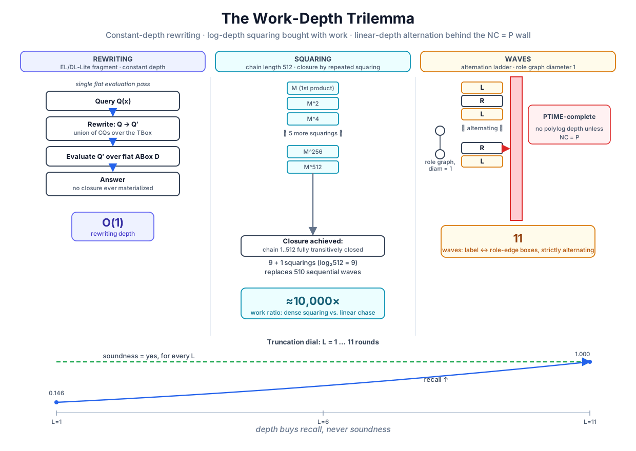Three lanes for three fragments: constant-depth rewriting, log-depth squaring bought with dense work, and the linear-depth alternating core behind the NC = P wall, with the truncation dial underneath trading recall, never soundness. Original diagram by the authors, created with AI assistance.

The table imposes a reading discipline this volume will enforce from here on: a reasoner's scalability is a property of the fragment before it is a property of the system. A benchmark result that says "system X materialized ontology Y in Z seconds" is uninterpretable until the fragment is named, because the same engine that flies on a preorder-shaped TBox must crawl, or truncate, on an alternation-shaped one. The diameter column of the committed reachability table and the $2k+1$ waves of the ladder are the same number wearing different fragments, and only the fragment says which kernel is even eligible.

Where the dial reappears

The truncation law is not a curiosity of this module; it is the load-bearing sentence of the volume's remaining parts, and each reappearance can now be named precisely. First, a fixed-depth neural network is a truncated kernel: a stack of $L$ layers is a computation whose depth is fixed at build time, so whatever iterative saturation it is asked to imitate, it can represent at most $L$ waves of it. The next chapter makes this exact for transformers, where the TC⁰ containment [3] plays the role the NC = P conditional played here. Second, chain-of-thought converts depth into serial decode steps: a model that writes intermediate conclusions into its own context and reads them back is running additional waves at inference time, paying for depth with tokens instead of layers; the chain-of-thought chapter measures that conversion on this volume's instruments. Third, the SATORI kernel's fixed-L unrolling (Part VII, the symbolic-attention chapter) is this chapter's law wearing attention weights: a symbolic-attention layer per completion wave, truncated at a build-time $L$, with a recall-versus-L table that is the committed curve above re-measured inside a neural architecture, and the same guarantee to defend, soundness at every budget.

The unsolved part

The chapter counted two axes and priced one trade, but the honest accounting has three axes, which is why the title says trilemma. Memory is the axis the module counted only implicitly: the squaring kernel's intermediate $A_t$ is a dense $n \times n$ matrix regardless of how sparse the closure is, and each squaring materializes a full dense product before comparing it to its input. At the module's $n = 512$ that is $262{,}144$ cells per intermediate, trivial; at a SNOMED CT-sized $n$ of several hundred thousand concepts it is on the order of $10^{11}$ cells per intermediate, which exhausts memory long before the $n^3$-flavored work exhausts patience. Squaring's dense intermediates blow memory before they blow work, so the real engineering frontier is a three-way negotiation among work, depth, and residency, and the module's clean two-column table deliberately does not capture it (its docstring concedes the dense kernel is float32 matmul at toy $n$, not a real subcubic algorithm; work_depth.py, lines 44–48). Second, crossover points are governed by constants no asymptotic captures: the committed ratios ($78.4$x at $n = 8$, $10{,}270$x at $n = 512$) count semiring operations, but wall-clock crossover depends on memory bandwidth, sparsity structure, and batch shape, which is precisely why the module reports counted operations and refuses to print timings (lines 50–51). Third, and most open: everything in this chapter used a fixed schedule, all-waves or all-squarings or a fixed budget $L$. A depth-adaptive reasoner would spend rounds where the instance needs them, detecting on the fly that this TBox is preorder-shaped (square it) and that one is alternation-shaped (wave it), or stopping a truncated run early with a certificate that the frontier is empty. Anytime kernels with per-instance depth certificates have, to date, been measured nowhere at scale, and the chapter's tables are exactly the kind of instrument such a measurement would need.

Why it matters

This chapter is the pivot on which Part IV hands the volume to Part V. Everything before it asked how to make a round of reasoning cheap: batching, deltas, tensors, rewriting. This chapter asked how many rounds must happen in order, and found the answer is a property of the logical fragment, defended by one of complexity theory's standard conjectures, and negotiable only in one currency: recall. That reframing does concrete work for a researcher. It says a scaling claim without a fragment is not a claim; it says a fixed-depth architecture evaluated on a reasoning benchmark has a ceiling that is knowable before training, by measuring the benchmark's derivation depth; and it says the safe way to spend a limited depth budget is the truncated kernel's way, keeping soundness and surrendering recall, because the opposite trade, keeping coverage and surrendering precision, is the one that later needs calibration machinery to repair. For the series arc, the sentence "depth buys recall, never soundness" is the bridge on which the transformer ceiling, chain-of-thought, and the SATORI kernel all stand; the reader who has watched the recall column climb while the soundness column stays pinned owns that sentence as a measured fact, not a slogan.

Key terms

• Work: the total number of operations a computation performs, summed over all processors; the bill someone always pays, in energy and hardware, whatever the clock says.
• Depth: the length of the longest chain of operations in which each needs its predecessor's result; a lower bound on running time for any number of processors.
• Brent's scheduling bound: with $p$ processors, greedy scheduling runs a computation of work $W$ and depth $D$ in time at most $W/p + D$, matching the two lower bounds $W/p$ and $D$ up to their sum.
• Semi-naive (wave) closure: the frontier discipline that joins only the newest facts against the base each round: depth $D - 1$ rounds, sparse output-proportional work, $(n-1)^2$ counted operations on the $n$-chain.
• Repeated squaring: closing reachability by squaring $I \vee M$: depth $\lceil \log_2 D \rceil$ productive rounds plus one confirming round, at $n^2(2n-1)$ dense counted operations per round.
• NC / NC²: the problems solvable by uniform circuit families of polynomial size and polylogarithmic depth; NC² allows depth $O(\log^2 n)$, and transitive closure lives there.
• P-completeness: membership in PTIME plus hardness for all of PTIME under logspace reductions; the formal notion of "inherently sequential", since a polylog-depth, polynomial-work algorithm for any P-complete problem would collapse NC = P.
• Alternation ladder: the gadget whose label derivations and edge derivations strictly interleave, forcing $2k+1$ waves over a role graph of diameter 1: derivation depth without reachability depth.
• Truncation law: a monotone saturation kernel stopped after $L$ rounds is sound at every $L$ and complete exactly at $L = D$, the instance's derivation depth: depth buys recall, never soundness.
• Diameter versus derivation depth: the graph quantity squaring can compress versus the dependency quantity it cannot; conflating them is exactly the strawman's mistake.

Where this leads

The trilemma was run on kernels this volume wrote and can inspect. The next chapter aims the same instrument at a kernel nobody hand-writes: the transformer, whose depth is fixed the day its config file is committed. The Transformer Depth Ceiling states the TC⁰ containment for fixed-depth, log-precision attention stacks, connects it to the P-completeness wall met here, and then does what this volume always does with an imported theorem: builds the committed toy that shows the ceiling behaving exactly as the theory predicts, a fixed-depth model failing on instances whose derivation depth exceeds its layers, with the truncation law's recall curve reappearing where a loss curve used to be.

---

Companion code: examples/frontier/work_depth.py implements all three tiers with counted work and depth: the semi-naive and squaring closures asserted against an independent DFS reference on the chain family and the academic ⊑-preorder, the alternation ladder and two-hop gadget asserted against Volume 2's el_completion oracle, the constant-round strawman's undershoot and overshoot asserted exactly, and the fixed-L truncation table asserted sound at every budget. Run python3 examples/frontier/work_depth.py to reproduce every number in this chapter.