The Transformer Depth Ceiling: TC⁰ and P

📍 Where we are: Part V · Neural Depth: Chain-of-Thought and RL (reinforcement learning) — Chapter 12. The Work-Depth Trilemma priced every computation on two axes, total work and unavoidable sequential depth, and found reasoning fragments that refuse to trade one for the other; this chapter aims that ruler at the dominant neural architecture and reads off its depth budget.

The previous chapter closed with a warning that its law would reappear in different clothes, and the first outfit is the transformer itself. A transformer applies $L$ layers, one after another, to all positions of its input at once. Everything about its scale lives in the width: more positions, wider embeddings, more attention heads, more parameters per layer. The one number that does not grow is $L$. In the vocabulary of the work-depth chapter, a transformer is a machine with enormous work and constant depth, and the trilemma says constant depth is not a free choice: it is a claim about which functions the machine can compute at all. This chapter states the theorem family that makes the claim exact, with the house discipline for imported theory: the results place log-precision transformers inside the constant-depth threshold-circuit class TC⁰, so any problem outside TC⁰ is beyond every fixed-depth transformer, at any parameter count, under separations whose status we state honestly. The companion module depth_ceiling.py then supplies what a toy can legitimately supply, which is the mechanism rather than the theorem: fixed-depth networks trained on short instances of two depth-carrying tasks generalize inside their training band and collapse to chance beyond a cliff, and extra depth pushes the cliff outward without ever removing it.

The simple version

Imagine a factory line with exactly three stations. Each station can hold ten thousand workers side by side, and every product on the belt is worked on simultaneously, so the line is staggeringly fast. But a product visits each station once, in order. Any recipe that genuinely needs four consecutive steps, where step four must see the result of step three, cannot be finished in one pass, and hiring more workers changes nothing, because the workers at station one cannot perform step four before steps two and three exist. That is a transformer: the stations are layers, the workers are width, and recipes whose number of dependent steps grows with the size of the order will eventually not fit, no matter the headcount. There are exactly two ways out. Rebuild the factory with more stations before the order arrives (more depth), or send the half-finished product around the line again and again (serial decoding). The next chapter is about the second way.

What this chapter covers

• The shape of the machine: why a transformer's parameters buy width rather than depth, and how the previous chapter's work-depth vocabulary turns "how many layers" into "what complexity class."
• Threshold circuits from scratch: Boolean circuit families, the classes AC⁰ and TC⁰ with every symbol decoded, what "uniform" rules out, and a full worked construction putting PARITY inside TC⁰ with counting gates.
• The ceiling theorem, imported with discipline: log-precision transformers without intermediate decoding lie in uniform TC⁰; the precise statement, the attribution, why the proof is beyond this volume, and what the companion demonstrates instead.
• The attention ladder: saturated and averaging attention reach MAJORITY and TC⁰, hard unique attention stays inside AC⁰, and PARITY separates the rungs unconditionally, so the attention nonlinearity is itself a complexity choice.
• The committed cliffs: depth-1/2/3 networks trained on lengths 2 through 6 and tested on 2 through 16; the per-depth accuracy tables, the cliff statistic derived, the asserts that guard every reading, and the honest statement of what the toy does and does not show.
• The series' own objects sorted: Volume 1's closure waves, Volume 2's PTIME-complete completion, Volume 3's role-chain ceiling, and this chapter's two tasks, each placed above or below the TC⁰ line, in one table.
• The two lanes out: exponential width, which is a payment and not an architecture, and serial decoding, which converts depth into time and is the next chapter's theorem.

The shape of the machine: width without depth

Recall the architecture from Volume 3's attention chapter. A transformer layer takes the current representation of every position, computes attention scores between all pairs of positions, mixes values by those scores, and pushes each position through a small feed-forward network. Nothing in that description is sequential across positions: position 17 does not wait for position 16. The only sequential axis is the layer index. An input of length $n$ (the number of tokens, our recurring size parameter) passes through layer 1, then layer 2, up to layer $L$, and $L$ is an architectural constant fixed before training, typically a few dozen, never a function of $n$. Scaling a model from millions to hundreds of billions of parameters multiplies the width of every matrix and the number of heads; it multiplies $L$ by a small constant at most. The shape is deliberate, because the parallelism across positions is exactly what makes training tractable on the hardware of the GPU chapter: every layer is a handful of dense matrix products, the ideal batched workload.

The work-depth chapter gives us the right question to ask about that shape. One layer performs a bounded number of dependent stages (a score computation, a normalization, a mix, a feed-forward pass), so the longest chain of operations in which each needs its predecessor's output has length proportional to $L$: constant in $n$. The work per layer is enormous, order $n^2$ attention scores alone, and grows freely. So a transformer occupies the extreme corner of the previous chapter's map: maximal work, constant depth. The trilemma's lesson was that some problems refuse to live in that corner, because their required depth grows with input size. The question this chapter answers precisely is: which problems? What, exactly, does constant depth buy? The answer is a circuit class, and the theorem that names it is the ceiling of this chapter's title [1].

Threshold circuits: the currency of constant depth

To state the theorem we need its vocabulary, built from the ground up. A Boolean circuit is a directed acyclic graph of gates: input nodes carry the bits $x_1, \ldots, x_n$ of the input, internal gates compute functions of their incoming wires, and one designated gate is the output. The size of a circuit is its number of gates; the depth is the length of the longest path from an input to the output, the circuit analogue of the previous chapter's dependent-chain count. A single circuit has a fixed number of inputs, so to compute a function of arbitrary-length inputs we use a circuit family: one circuit $C_n$ for each input length $n$, where the subscript $n$ names the length that circuit handles.

Two constant-depth classes matter here. AC⁰ is the class of problems solvable by circuit families of constant depth (the same depth bound for every $n$) and polynomial size (the gate count of $C_n$ grows at most like $n^c$ for some fixed constant exponent $c$), using NOT gates and AND/OR gates of unbounded fan-in, meaning a single AND or OR may read any number of wires at once. TC⁰ keeps the constant depth and polynomial size but adds one more gate type, the threshold gate: for a threshold $\theta$ (an integer parameter of the gate), the gate $\mathrm{Th}_{\ge \theta}$ outputs 1 exactly when at least $\theta$ of its input wires carry 1. In symbols, with $\sum_{i=1}^{m} x_i$ denoting the ordinary integer sum of the $m$ input bits,

$$\mathrm{Th}_{\ge \theta}(x_1, \ldots, x_m) = 1 \quad \text{exactly when} \quad \sum_{i=1}^{m} x_i \ge \theta.$$

A threshold gate can count; an AND/OR gate can only detect all-or-any. The special case $\theta = \lceil m/2 \rceil$ (the ceiling brackets $\lceil \cdot \rceil$ round up to the next integer) is the MAJORITY gate, which fires when at least half its inputs do, and MAJORITY is complete for the class in the sense that TC⁰ is unchanged if threshold gates are replaced by MAJORITY gates. One more qualifier appears in every serious statement: uniform. A circuit family is a different object for every $n$, and without a constraint the family could smuggle uncomputable knowledge into its wiring, one hard-coded answer per length. A family is uniform when a single simple algorithm (logarithmic-space is the standard choice) outputs the description of $C_n$ given $n$. Uniformity turns "a family of circuits exists" into "one finite recipe builds them all," which is what a fixed transformer with fixed weights actually is.

To see what the threshold gate buys, we can afford a full construction, because this one the chapter owns. PARITY is the function on $n$ bits that outputs 1 exactly when an odd number of them are 1. Build an exactly-$k$ detector from two threshold gates: with $m$ the number of ones in the input,

$$E_k(x) = \mathrm{Th}_{\ge k}(x) \wedge \neg\, \mathrm{Th}_{\ge k+1}(x),$$

where $\wedge$ is AND and $\neg$ is NOT. Check it against the definition: $\mathrm{Th}_{\ge k}$ fires exactly when $m \ge k$, and $\neg\,\mathrm{Th}_{\ge k+1}$ fires exactly when $m \le k$, so the conjunction fires exactly when $m \ge k$ and $m \le k$ hold together, that is, when $m = k$ precisely. Now sum over the odd counts with an unbounded fan-in OR (the symbol $\bigvee$ below is an OR over all the listed cases):

$$\mathrm{PARITY}(x) = \bigvee_{k \text{ odd},\; 1 \le k \le n} E_k(x).$$

The disjuncts are mutually exclusive (the count $m$ has one value), so the OR is exact. Count the resources: at most $n + 1$ threshold gates on the first level, at most $n$ AND/NOT pairs on the second, one OR on the third; size linear in $n$, depth 3, for every $n$. PARITY is therefore in TC⁰, by a circuit you can draw. Hold that construction in mind, because the deepest unconditional fact in this chapter is that without threshold gates it is impossible: no constant-depth polynomial-size AND/OR/NOT family computes PARITY. That separation arrives two sections below with its citation, where the ladder needs it. The known inclusion chain, each class allowing more depth, reads

$$\mathrm{AC}^0 \subseteq \mathrm{TC}^0 \subseteq \mathrm{NC}^1 \subseteq \mathrm{NC}^2 \subseteq \mathrm{P},$$

where $\subseteq$ means "is contained in," NC¹ and NC² are the classes with depth allowed to grow like $\log n$ and $\log^2 n$ (with bounded fan-in gates), and P is polynomial time, the home of the previous chapters' completion procedures. Which of these containments are strict is mostly unknown; the single strictness this chapter uses unconditionally is the first one, and everything to the right of TC⁰ is conjecture, flagged as such wherever it bears weight.

The ceiling theorem, imported with discipline

One more decoded term and the theorem can be stated. A transformer is log-precision when every number in its forward pass at input length $n$ (activations, attention scores, partial sums) is stored in $O(\log n)$ bits, meaning at most $c \log_2 n$ bits for some fixed constant $c$. Decode the consequence: $c \log_2 n$ bits distinguish at most $2^{c \log_2 n} = n^c$ values, so every intermediate quantity ranges over polynomially many possibilities. This is the honest idealization of practice, where 16- or 32-bit floats are constants that comfortably exceed $\log_2 n$ for real context lengths, and it is the assumption that keeps a single activation from hiding an unbounded amount of information.

The theorem [1]: any transformer with a fixed number of layers, polynomially bounded size, and log-precision arithmetic, run as a single forward pass that outputs its answer directly (no intermediate tokens generated and fed back), recognizes only languages in logspace-uniform TC⁰.

Every quantifier in that sentence is load-bearing. "Any transformer" means the bound is architectural: it holds for every setting of the weights, so no training run, however long, escapes it. "Fixed number of layers" is where constant depth enters. "No intermediate tokens" reserves the escape hatch that the next chapter opens. The proof is genuinely beyond this volume, but its shape can be said in one honest paragraph: with log-precision values there are only polynomially many distinct numbers in play, and the arithmetic a layer performs on them, iterated addition of $n$ numbers, multiplication, and the division inside the softmax normalization, are all classical TC⁰ primitives, computable by constant-depth threshold circuitry; each layer therefore simulates in constant depth, the $L$ layers stack to $L$ times a constant, still a constant, and a careful uniformity argument checks that one logspace algorithm can emit the whole simulating family [1]. What this chapter's companion demonstrates is not that argument, and nothing in this volume should be read as proving it; the companion demonstrates the mechanism the theorem formalizes, on models small enough to watch.

The attention ladder: architecture choices are complexity choices

The TC⁰ ceiling is one rung of a ladder, and the ladder's lesson is worth the two extra results, because it shows the circuit class responding to a single architectural dial: what the attention nonlinearity does with its scores.

Saturated attention reaches TC⁰ and MAJORITY. Saturated attention is the zero-temperature limit of softmax: the attention weight spreads uniformly over the positions achieving the maximum score, exactly the averaging behavior real heads approach when scores separate sharply. Transformers with saturated attention and floating-point activations lie in TC⁰, and averaging attention computes MAJORITY directly, since an average over positions compared against a threshold is precisely a count compared against a threshold [2]. Averaging is counting, and counting is the threshold gate.

Hard unique attention stays inside AC⁰. Hard unique attention attends to exactly one position, the argmax with ties broken by position. Transformers built from it (the UHAT and GUHAT families, unique-hard-attention transformers and their generalized variant) recognize only languages in AC⁰ [3]: selecting one witness per head is an existential act that unbounded fan-in AND/OR circuitry can simulate, and no counting ever happens.

PARITY separates the rungs unconditionally. PARITY is not in AC⁰: no constant-depth, polynomial-size AND/OR/NOT circuit family computes it, one of the few lower bounds in complexity theory that needs no conjecture [4]. MAJORITY is not in AC⁰ either, since a constant-depth circuit with majority gates available computes parity (the construction one section back), so parity's impossibility lifts to majority. The two rungs are therefore genuinely different floors: a hard-attention transformer provably cannot count bits mod 2 at all lengths, while a saturated-attention transformer sits a strict level up, able to count but, by the ceiling theorem, no further. A broad survey maps many more variants onto this ladder, with positional encodings, precision regimes, and masking each moving the class [5]. The reading that matters for this series: the nonlinearity in attention is a complexity-class choice. Deciding between argmax selection and averaging is not a hyperparameter tweak; it decides whether the architecture can count at all.

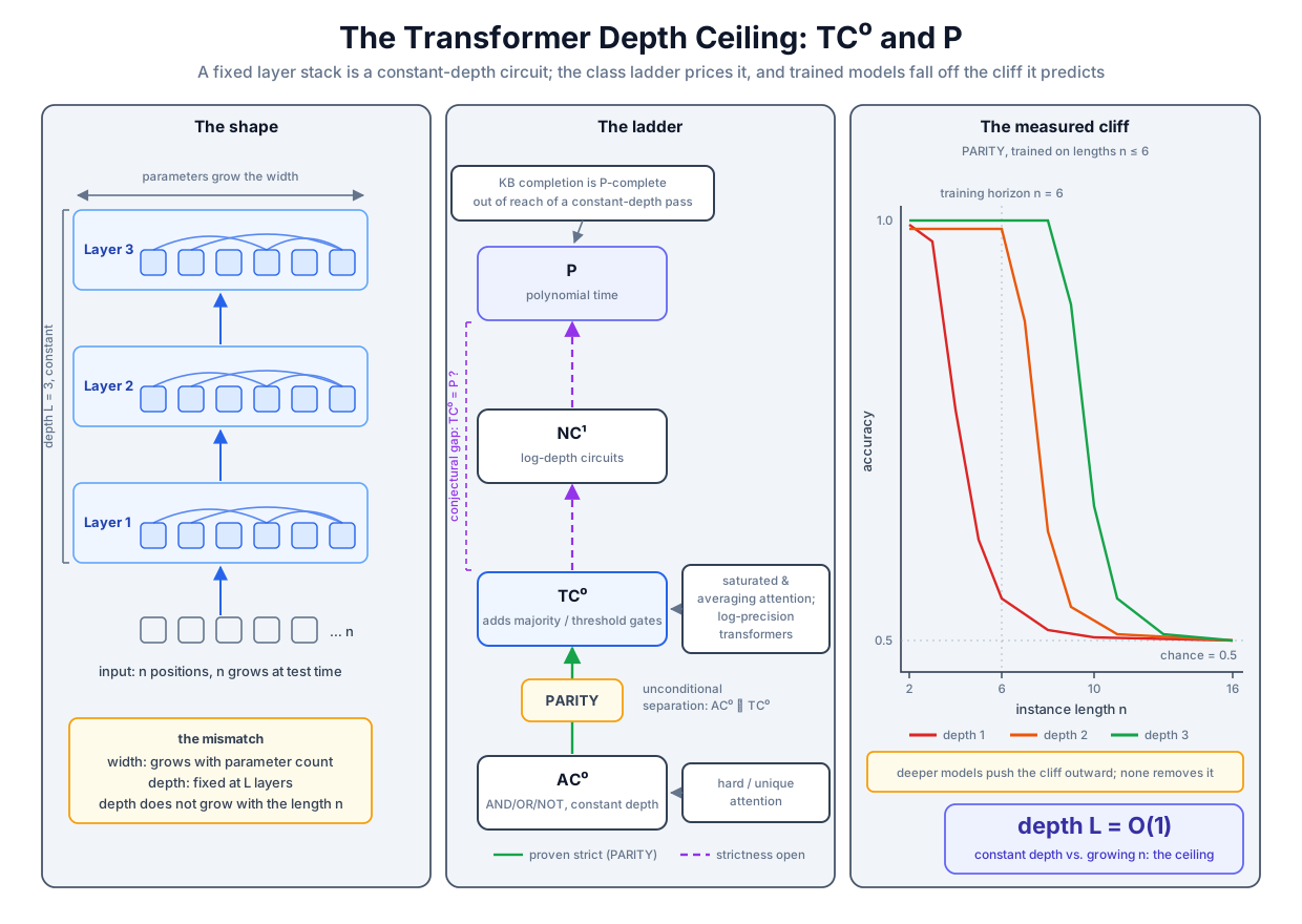The constant-depth shape, the circuit-class ladder that prices it, and the committed length-generalization cliffs that show the mechanism on trained models. Original diagram by the authors, created with AI assistance.

What the ceiling excludes: the series' objects sorted

The corollary that gives the chapter its title is now one containment chase. Suppose a fixed-depth log-precision transformer decided a P-complete problem, one to which every polynomial-time problem reduces in logarithmic space; the previous chapter's Datalog closure and Volume 2's EL completion are the running examples. By the theorem, the problem would lie in logspace-uniform TC⁰, and uniform TC⁰ sits inside logspace itself (a logspace machine can build and evaluate a constant-depth circuit on the fly). Composing the reductions would put all of P inside logspace, hence inside NC² (a classical simulation: a logspace machine has only polynomially many configurations, and reachability over that configuration graph is computable by circuits of depth $\log^2 n$), and the entire chain from TC⁰ to P would collapse to its bottom rungs: P = NC, every polynomial-time computation parallelizable to polylogarithmic depth. That collapse is exactly the disbelieved-but-unproven possibility the previous chapter flagged. So the precise statement is conditional and honest: unless the hierarchy collapses, no fixed-depth transformer of any size decides a P-complete problem at all input lengths. Contrast the status of the two separations this chapter leans on: PARITY outside AC⁰ is a theorem with no conditions [4]; TC⁰ strictly below P (indeed, TC⁰ strictly below NC¹) is a conjecture, universally believed, never proved. The house rule is to say which is which, every time.

With the ceiling priced, this series' own computations sort themselves. Each row below is an object the reader has already run; the class column is the problem's home, and the verdict column asks whether a fixed-depth transformer could in principle represent it at all input scales.

Computation (where it lives in the series)	Complexity home	Under the TC⁰ ceiling?
Degree counting, MAJORITY-style aggregation (Volume 3's attention pooling)	TC⁰	Inside: counting is the threshold gate.
PARITY of $n$ bits (this chapter's task)	TC⁰, outside AC⁰ [4]	Inside TC⁰, but above the hard-attention rung.
Iterated $S_3$ composition (this chapter's task)	Inside TC⁰ unconditionally: solvable-group word problems sit in ACC⁰ ⊆ TC⁰, where ACC⁰ is AC⁰ with modular-counting gates added (Barrington–Thérien [6])	Inside as a function family: a mechanism testbed, not a separation witness.
Iterated $S_5$ composition	NC¹-complete (Barrington's theorem [7])	Outside unless TC⁰ = NC¹.
Reachability, atomic-subsumption closure (Volume 2; last chapter's squaring kernel)	NL-complete (NL is nondeterministic logarithmic space, the home of directed reachability), inside NC²	Outside unless TC⁰ swallows NL.
Volume 1's forward-chaining closure on the 23-fact knowledge base (KB), $D = 3$ waves	Constant depth for the fixed KB	Inside: a fixed instance needs only fixed depth.
Datalog / EL completion as the KB grows (Volume 2; the trilemma chapter)	P-complete	Outside unless P = NC.
Role-chain axiom checking by message passing (Volume 3's ceiling)	Needs three variables, beyond C² (the two-variable counting logic of Volume 3's ceiling)	The graph-neural-network (GNN) analogue: a fixed-round ceiling of its own.

Two rows deserve a pause. Volume 1's closure ran in $D = 3$ waves because the academic KB is 23 facts; a fixed-depth network genuinely can represent any fixed number of waves, which is why small benchmarks routinely feel like counter-evidence to the theory. The ceiling binds the family: as the KB grows, the required wave count grows, and no constant $L$ covers all of it. And the $S_3$ row is a deliberate honesty exhibit. Group theory calls a group solvable when it can be built up from commutative pieces (a term of art, distinct from this chapter's earlier everyday sense of a problem being solvable by circuits); $S_3$ is solvable, $S_5$ is not. That property settles the row: the word problem of a solvable group, the task of naming an iterated product, lies inside TC⁰ unconditionally by the Barrington–Thérien fine-structure theorem [6], so $S_3$ can never witness the separation, while for the non-solvable $S_5$, iterated composition is NC¹-complete by Barrington's theorem [7], hence outside TC⁰ unless the conjectured separation fails. The companion chose $S_3$ anyway, and the module's docstring says why in advance (depth_ceiling.py, lines 30–38): what the experiment needs is not a class separation but a depth knob, a task whose required chain of dependent operations grows with instance length. Both tasks have exactly that, and neither experiment will be sold as more.

What a toy can honestly show

The house rule for imported theory has a corollary for companion code, and this module performs it in prose before printing a single number (depth_ceiling.py, lines 59–66): the cited theorems bound the expressiveness of log-precision transformers, meaning which functions a fixed-depth network can represent at all; a small trained MLP (multilayer perceptron, a stack of fully connected layers) exhibits the empirical shadow of that ceiling, a length-generalization cliff whose position grows with depth, and not the circuit-class separation itself. Finite experiments illustrate; they do not prove. Both tasks are also within TC⁰, as the table just recorded, so what the laboratory isolates is the mechanism the theorems formalize: a network with $L$ rounds of nonlinearity has $L$ chances to combine information, and a task whose instances need a growing number of dependent combination steps must eventually fall off any fixed $L$, at least for the solutions gradient descent actually finds from short training instances. The run itself prints the same disclaimer as its first act, and the block below is committed output, not paraphrase:

[1] the theory ladder (imported results, cited, never re-proved here)
    unique/generalized hard attention (UHAT/GUHAT) ⊆ AC⁰  [Hao, Angluin & Frank, TACL 2022]
      (averaging hard attention, AHAT, computes MAJORITY ∉ AC⁰: it sits in TC⁰)
    PARITY ∉ AC⁰                                          [Furst, Saxe & Sipser 1984; Håstad 1986]
    saturated attention ⊆ TC⁰                             [Merrill, Sabharwal & Smith, TACL 2022]
    log-precision transformers ⊆ uniform TC⁰              [Merrill & Sabharwal, TACL 2023]
    no CoT: only TC⁰  /  poly-step CoT: P                 [Merrill & Sabharwal, ICLR 2024]
    (theorems about transformer expressiveness; the MLPs below are the lab analogue)

Task one: iterated $S_3$ composition, because composition carries depth. $S_3$ is the symmetric group on 3 letters: the 6 permutations of $(0, 1, 2)$, listed in lexicographic order so that element 0 is the identity, with composition $(\sigma_a \circ \sigma_b)(x) = \sigma_a(\sigma_b(x))$, the right factor acting first (depth_ceiling.py, lines 90–102). An instance of length $n$ writes $n$ uniformly random non-identity elements into the first $n$ of 16 input slots, pads the rest with the identity, and asks for the product, a 6-way classification (lines 105–138). Why is composition the depth carrier? Because the defining evaluation is a chain in which every step consumes the previous step's output. The module computes the label by exactly that left fold (lines 111–117):

def s3_product(elems: np.ndarray) -> np.ndarray:
    """Row-wise product of a (count, n) matrix of element ids, folded left to
    right through the Cayley table: p_0 = e;  p_j = p_{j-1} ∘ g_j."""
    prod = np.zeros(len(elems), dtype=np.int64)
    for j in range(elems.shape[1]):
        prod = MUL[prod, elems[:, j]]
    return prod

That fold is $n - 1$ dependent multiplications for $n$ non-trivial factors: depth linear in $n$. Associativity lets a smarter schedule regroup, exactly as the previous chapter's balanced tree regrouped a sum: pair adjacent factors and multiply all pairs at once, leaving $\lceil n/2 \rceil$ factors, and repeat; after $t$ rounds at most $\lceil n / 2^t \rceil$ factors survive, so one survives after $t = \lceil \log_2 n \rceil$ rounds. Depth logarithmic in $n$ is the floor for schedules built from group multiplications, and any function of $n$ that a network computes in a constant number of combination rounds must shortcut both schedules. Furthermore, PARITY embeds in this family, and the embedding is a two-line derivation the module asserts rather than assumes. Let $\tau$ be the transposition that swaps letters 0 and 1 and fixes 2. Composing it with itself returns every letter to its place, so $\tau \circ \tau = e$, the identity; by induction, a product of $n$ copies of $\tau$ equals $e$ when $n$ is even (pair the factors off) and $\tau$ when $n$ is odd (one factor survives the pairing). Whoever can name the product of $n$ transpositions has computed $n \bmod 2$. The harness checks the group table exhaustively, associativity, inverses, non-commutativity, and this order-2 identity, before any training runs (depth_ceiling.py, lines 332–343).

Task two: PARITY on weight slices, the classical witness. An instance of length $n$ places exactly $n$ ones at uniformly random positions of a 16-bit string and asks for $n \bmod 2$: PARITY on the Hamming-weight-$n$ slice of $\{0,1\}^{16}$ (lines 141–161), the very function the unconditional AC⁰ lower bound is about [4]. Here the depth knob and the class witness coincide, and the label depends on every bit: flip any one and the answer flips.

The committed demonstration instances make both encodings concrete (real output):

[2] the two task families — the depth knob is the length n
    S_3 as image words (0 is the identity): 0:012  1:021  2:102  3:120  4:201  5:210
    iterated composition, n=4:  201 ∘ 210 ∘ 021 ∘ 210  =  021   (class 1; rightmost factor acts first)
    weight-slice parity, n=5:   0110011001000000   →  parity 1 (odd number of ones)

The laboratory models. The trained objects are MLPs of depth 1, 2, and 3, where depth counts tanh (hyperbolic tangent) hidden layers of a fixed width, with a softmax cross-entropy head; every gradient is hand-derived, the same $\delta$-recursion this series built in Volume 1, implemented in loss_and_grads (depth_ceiling.py, lines 191–224) and driven by minibatch stochastic gradient descent (SGD) with heavy-ball momentum (lines 227–248). Decode the two formulas the loss_and_grads docstring records, writing $\mathcal{L}$ for the training loss (the docstring writes it $L$; this chapter reserves $L$ for the layer count), $z$ for the pre-softmax scores, $P$ for the matrix of predicted class probabilities (a matrix here, not the complexity class), $Y$ for the one-hot true labels, $B$ for the batch size, $l$ for the layer index, $W_l$ for layer $l$'s weight matrix with $W_l^\top$ its transpose, $a_{l-1}$ for the previous layer's activations, $\odot$ for the entry-wise product, and $\delta_l$ for the error signal arriving at layer $l$: the softmax cancellation reads $\partial \mathcal{L}/\partial z = (P - Y)/B$, and the tanh backward rule reads $\delta_{l-1} = (\delta_l W_l^\top) \odot (1 - a_{l-1}^2)$. Before the experiment is allowed to mean anything, the arithmetic is certified: with $\theta$ now standing for the network's flattened parameter vector (a second life for the letter, unrelated to the threshold gate's integer parameter) and $h$ a small probe step, every analytic partial derivative of a small float64 depth-3 net is compared against the central finite difference $(\mathcal{L}(\theta + h) - \mathcal{L}(\theta - h))/(2h)$, and the worst relative gap in the committed run is $2.1 \times 10^{-11}$, guarded by an assert at $10^{-6}$ (lines 256–279 and 346–347). Whatever the cliffs mean, they are not a backprop bug.

The protocol. Training sees only short instances, $n = 2$ through $6$ (600 per length for parity, 2000 for $S_3$); evaluation draws fresh instances at every length $n = 2$ through $16$, 400 per length (lines 83–86, 287–292, and 295–303). The control is stated in the code rather than left implicit: within a task family, one protocol dictionary fixes the hidden width (32 for parity, 40 for $S_3$), learning rate, epoch count, batch size, and both data and model seeds, and only the depth varies between the three models, with one honest caveat: the per-model random seed is the task's fixed model seed offset by the depth (depth_ceiling.py, lines 284–292 and 358), since architectures of different sizes cannot share one initialization anyway. The module contains no width sweep, so it attributes the coming displacement to depth on ceteris-paribus grounds: three models per task, identical in everything but $L$ and the seed offset it fixes.

The committed cliffs, read carefully

One statistic condenses each accuracy-versus-length row before we read the rows themselves. With chance accuracy $c$ (here $c = 1/2$ for parity's two classes, $c = 1/6 \approx 0.167$ for $S_3$'s six), define the cliff position as the largest $n$ such that accuracy stays at or above the midpoint $(1 + c)/2$, halfway between perfect and chance, at every length from 2 up to $n$ (depth_ceiling.py, lines 306–316):

def cliff_length(accs: dict[int, float], chance: float) -> int:
    """The cliff position: the largest n such that accuracy stays at or above
    the midpoint (1 + chance)/2 — halfway between perfect and chance — at
    EVERY length 2..n.  Returns 1 if even n = 2 is below the midpoint."""
    midpoint = (1.0 + chance) / 2.0
    last = 1
    for n in EVAL_LENGTHS:
        if accs[n] < midpoint:
            break
        last = n
    return last

The midpoints are $0.750$ for parity and $(1 + 1/6)/2 = 7/12 \approx 0.583$ for $S_3$. The "every length up to $n$" clause matters: a row that recovers after a dip does not get credit for the recovery, because a model that fails at $n = 4$ has already fallen off the task. Here are both committed tables, verbatim; the vertical bar marks the training horizon $n = 6$:

[4] PARITY on weight slices (chance 0.500, cliff midpoint 0.750)
      accuracy vs length; '|' marks the training horizon n = 6
        n:      2    3    4    5    6 |    7    8    9   10   11   12   13   14   15   16   train  cliff
  depth 1  1.00 0.97 0.58 0.45 0.87 | 0.08 0.98 0.00 1.00 0.00 1.00 0.00 1.00 0.00 1.00   0.900      3
  depth 2  1.00 1.00 1.00 1.00 1.00 | 0.00 1.00 0.00 1.00 0.00 1.00 0.00 1.00 0.00 1.00   1.000      6
  depth 3  1.00 1.00 1.00 1.00 1.00 | 0.00 1.00 0.00 1.00 0.00 1.00 0.00 1.00 0.00 1.00   1.000      6

[5] iterated S_3 composition (chance 0.167, cliff midpoint 0.583)
      accuracy vs length; '|' marks the training horizon n = 6
        n:      2    3    4    5    6 |    7    8    9   10   11   12   13   14   15   16   train  cliff
  depth 1  1.00 1.00 0.96 0.64 0.47 | 0.10 0.17 0.15 0.14 0.17 0.18 0.19 0.17 0.16 0.20   0.883      5
  depth 2  1.00 1.00 0.98 0.80 0.47 | 0.12 0.17 0.18 0.15 0.12 0.17 0.17 0.17 0.16 0.17   0.995      5
  depth 3  1.00 1.00 0.99 0.81 0.52 | 0.12 0.20 0.16 0.19 0.16 0.14 0.16 0.13 0.15 0.14   0.985      5

Read the parity table first, and start inside the training band. Depth 1 never masters its own band: accuracy dips to $0.58$ at $n = 4$ and $0.45$ at $n = 5$, both below the $0.750$ midpoint, so its cliff sits at $n = 3$, inside the lengths it was trained on. One tanh layer of width 32 could not even fit the depth-5 dependency structure it saw during training. Depths 2 and 3 are perfect across the whole band, cliff at the horizon $n = 6$. That displacement, cliff at 3 for depth 1 versus 6 for depth 2, is the experiment's cleanest sentence, and it is guarded as code rather than prose: the harness asserts that depth 1 cliffs at or before $n = 4$, that depth 2 reaches exactly the horizon, and that depth 2 strictly out-generalizes depth 1 (depth_ceiling.py, lines 389–394), along with the general monotonicity claim that the cliff position never decreases with depth on either task (lines 383–385).

Beyond the horizon the parity rows alternate between $0.00$ and $1.00$, and this pattern is worth deriving rather than gawking at, because it dictates what the honest collapse statistic is. On a weight-$n$ slice, every test instance of a given length carries the same label, $n \bmod 2$. A network pushed far outside its training distribution saturates and answers a nearly constant class; a constant answer scores accuracy 1 at lengths whose true label happens to match and 0 at lengths where it does not, alternating with $n$. So per-length accuracy out there is uninformative on its own: the $1.00$ at $n = 10$ is not generalization, it is a stopped clock agreeing with the calendar twice a day. The honest statement is the average over the tail lengths $n = 7$ through $16$, which contain five odd and five even values, so a constant-answer model averages to exactly $0.5$, chance. The committed tails are $0.506$, $0.500$, and $0.500$ for depths 1, 2, 3, and the harness asserts every tail is within $0.12$ of chance while every model masters length 2 at $0.90$ or better and its training set at $0.80$ or better (lines 370–382): the collapse is real, and it is a collapse of a model that demonstrably learned the short version of the task.

The $S_3$ table tells the same story with a different accent. All three depths cliff at $n = 5$; the position ties at this scale. But depth is still visible exactly where the theory says it should be, at the deepest trained length: accuracy at $n = 5$ climbs $0.64 \to 0.80 \to 0.81$ from depth 1 to 2 to 3, a strict gain guarded by asserts requiring at least five points of improvement (lines 397–401). Beyond the horizon the tails are $0.162$, $0.157$, $0.155$ against chance $0.167$: six-way chance, no alternation artifact, straightforward collapse. And no row anywhere in either table has a cliff beyond $n = 6$. The summary line commits every number this chapter has quoted:

SUMMARY depth_ceiling: parity_cliffs=3/6/6 s3_cliffs=5/5/5 parity_tail=0.506/0.500/0.500 s3_n5=0.64/0.80/0.81 fd_gap=2.1e-11

Now the reading discipline, which is the most important paragraph in the chapter. The theorems of this chapter are statements about a function class: they delimit which input-output mappings any fixed-depth architecture can represent, over all weight settings, at all input lengths. The tables above are statements about particular training runs: three seeds, two tasks, gradient descent from short instances. The two kinds of statement point in the same direction here, and that is precisely why the pairing is instructive, but neither implies the other. The cliffs cannot prove a lower bound (both tasks are inside TC⁰, and a wider or better-trained fixed-depth model could push any particular cliff further out); and the theorems did not predict the cliff positions (nothing in circuit complexity says depth 1 fails at $n = 4$ on 16-slot parity). What the toy shows is the mechanism that makes the theorems bite: a constant number of combination rounds is a real resource, models spend it, and when instances demand more of it than the model has, performance does not degrade gracefully, it falls off a cliff. What the theorems show is that above the toy, at the scale of the function family, no amount of training can buy the missing rounds. Keep the two sciences separate and both are useful; conflate them and you will either dismiss lower bounds because a benchmark improved, or dismiss a benchmark because a lower bound exists.

The two lanes out, and their prices

Nothing in this chapter says a fixed-depth network cannot approximate a hard task at bounded lengths, and the escape routes are exactly the two the factory analogy predicted.

Lane one: pay in width and precision. Every function on inputs of length $n$ is computable by a circuit of depth 2 and size exponential in $n$ (one gate per satisfying input, a disjunction over them), so a family of fixed-depth networks whose width explodes exponentially with length can memorize its way past any cliff. This is a payment, not an architecture: the polynomial-size condition in AC⁰ and TC⁰ is what makes them models of feasible parallelism, and a solution that doubles its hardware per added token has abandoned feasibility rather than beaten the ceiling. The lane matters because it calibrates benchmark claims; a fixed-depth model that solves lengths up to 16 may be spending width the way this lane spends it, and the only test is to grow $n$.

Lane two: pay in time, by decoding. The theorem's quietest clause was "no intermediate tokens." Let the transformer generate tokens and feed them back, and each generated token is a fresh forward pass whose input includes everything generated so far: a serial chain, depth converted into time, the factory sending the product around the line again. The module's printed ladder already contains the destination, quoted from the committed output above: with no chain of thought, only TC⁰; with polynomially many generated intermediate steps, exactly P. The next chapter states that theorem with this chapter's discipline, and its companion cot_steps.py imports this module's $S_3$ task machinery and MLP engine unchanged (depth_ceiling.py, lines 64–66) and breaks the $S_3$ cliff in the table above by spending steps instead of layers. The cliff-hanger is precise: the same task, the same training band, and a model that walks off the horizon without falling.

The unsolved part

The gap between the theory's idealizations and deployed models is real, two-sided, and open. The theorems assume log precision, uniformity, and clean attention limits (saturated averaging or hard argmax); a deployed model has finite everything, learned attention patterns that are neither limit, positional encodings the clean statements must be extended to cover, and a training procedure the theorems never mention. Inside that gap, empirical length generalization sometimes beats the pessimism a casual reading of the ceiling suggests, with the right scratchpad formats, positional schemes, or curricula stretching cliffs impressively far on particular task families, and sometimes underperforms it, with models failing at lengths the function class provably covers, exactly as this chapter's depth-1 parity model failed inside its own training band on a task that a one-hidden-layer network of sufficient width can represent perfectly at $n \le 6$. Both failures of prediction have the same root: expressiveness theory delimits which solutions exist, and says nothing about which solutions gradient descent finds. Characterizing the trained-solution class, the subset of the function class that optimization actually reaches from realistic data, and hence saying in advance which models the ceiling effectively binds at deployable scales, is an open problem where circuit complexity and learning dynamics are, today, different sciences with a shared vocabulary and no shared theorems.

Why it matters

This chapter is the series' two cultures meeting on the neural side's home ground. Volumes 1 and 2 built reasoners whose correctness proofs are induction over derivation depth: the closure exists because wave $k+1$ extends wave $k$. Volume 3 ended with a ceiling on message passing; this chapter is the same result-shape for the architecture that now mediates most machine reasoning, and it explains, before any benchmark is run, why a fixed-depth model that aces short logical inference falls off at depth, why parameter count does not rescue it, and why the failure arrives as a cliff rather than a slope. For the neuro-symbolic project the theorem family is close to a design brief: if the reasoning your system must perform is P-complete at scale, then the depth has to live somewhere other than the stack of layers, in a symbolic engine called as a tool, in a fixpoint loop wrapped around the network (the truncated kernel of the previous chapter, which is also SATORI's fixed-$L$ shape), or in the decode loop the next chapter analyzes. And for the reader's own research the chapter's last discipline is the transferable one: keep "the class cannot" and "this run did not" in separate columns of your notebook, because papers that blur them, in either direction, are the ones whose claims do not survive a change of $n$.

Key terms

• Circuit family / size / depth: one Boolean circuit $C_n$ per input length; gate count and longest input-to-output path; depth is the circuit form of the previous chapter's dependent-chain length.
• AC⁰: constant-depth, polynomial-size circuits with unbounded fan-in AND/OR and NOT; the home of hard unique attention; provably cannot compute PARITY.
• Threshold gate / MAJORITY: a gate firing when at least $\theta$ of its inputs are 1; majority is the $\theta = \lceil m/2 \rceil$ case; the gate that counts.
• TC⁰: AC⁰ plus threshold gates; the class containing log-precision fixed-depth transformers; contains PARITY by the exactly-$k$ construction.
• Uniformity: the requirement that one simple algorithm emits the whole circuit family, so the family is a finite recipe rather than an infinite table of hard-coded answers.
• Log precision: every value in the forward pass carries $O(\log n)$ bits at input length $n$, hence ranges over polynomially many possibilities.
• The ceiling theorem: fixed-depth, poly-size, log-precision transformers without intermediate decoding recognize only logspace-uniform TC⁰ languages, for every weight setting.
• Cliff position: the largest $n$ such that accuracy stays at or above the perfect-chance midpoint at every length up to $n$; the module's committed cliffs are 3/6/6 (parity) and 5/5/5 ($S_3$) for depths 1/2/3.
• Function class versus training run: the discipline separating what an architecture can represent (theorems, all weights, all lengths) from what one optimization found (experiments, one seed, one band); the toy illustrates the first and can only measure the second.

Where this leads

The ceiling theorem left one door explicitly open: it bounds a transformer that answers in a single forward pass, and says nothing about a transformer that talks to itself first. The next chapter, Chain-of-Thought: Recovering P at Decode Time, walks through that door with the same discipline, stating the ladder theorem (logarithmically many generated steps buy little, polynomially many reach exactly P), and its companion cot_steps.py re-runs this chapter's iterated $S_3$ task with a decode loop and watches its cliff disappear, at a price now denominated in the one currency the trilemma said was left: time.

---

Companion code: examples/frontier/depth_ceiling.py generates both task families, trains the depth-1/2/3 MLPs with hand-derived backprop certified against central finite differences (committed gap 2.1e-11), prints the accuracy-versus-length tables, and asserts the chapter's qualitative claims: training-band mastery, chance-level tails beyond the horizon, cliff monotonicity in depth, the parity displacement (depth 1 cliffs inside the band at or before n = 4, depth 2 reaches the horizon n = 6), and an at-least-five-point S₃ accuracy gain over depth 1 at n = 5 (the committed values are 0.64 → 0.80 → 0.81). Run python3 examples/frontier/depth_ceiling.py to reproduce every number; two runs print byte-identical output.