The SATORI Architecture: One Operator, Four Properties

📍 Where we are: Part VII · The SATORI Capstone — Chapter 19. Symbolic Attention built the operator: one weight-tied soft layer, unrolled a fixed number of times, that recovers Volume 1's forward chaining and Volume 2's EL completion exactly in its crisp limit. This chapter surrounds that operator with everything else a system needs, and holds every claim about the result to an instrument this volume already built.

An operator is not an architecture. The kernel of the previous chapter answers one question, how the two classical reasoners become a single differentiable pass, and leaves every other question open: what data structure the pass runs over, where its confidence numbers come from, how its rules could ever be learned rather than given, what its attention record is worth as an explanation, and what happens when the knowledge base stops being thirteen entities. SATORI's answer is a design with three parts: the operator, two substrates it runs over (an annotated rule representation and a box-embedding vocabulary), and one discipline (the derivation trace is a first-class output of the forward pass, never a story reconstructed afterward). From that assembly the project claims four properties: learnable routing, faithful traces, parallel scale, and calibrated open-world confidence. The claims are not the chapter's point. The point is the method by which they are made: every property is paired with an independent measuring instrument, each instrument was built and validated in an earlier Part of this volume before the architecture it now judges existed, and each verdict here is a committed number a script re-derives on every run.

The simple version

Imagine a startup pitching a machine that is fast, safe, efficient, and quiet. You can respond in two ways. You can listen to the pitch. Or you can bring your own stopwatch, your own crash rig, your own power meter, and your own microphone, none of them supplied by the startup, and measure. Whatever the machine turns out to be, the second response is the only one that produces knowledge. This chapter is the second response applied to a reasoning architecture, with one twist: we built the stopwatch, the rig, the meter, and the microphone first, across six Parts, and only now wheel the machine into the room. Each of the four advertised properties gets exactly one instrument, and the instrument, not the pitch, says what survives.

What this chapter covers

• The design problem as a wedge: three families of systems, each missing what another has (exact reasoners that cannot learn, rule learners blind to ontologies, embedders that neither prove nor calibrate), and the architecture's bet that one operator over the right substrates occupies all corners at once.
• Substrate one, the annotated ontology IR (intermediate representation): every axiom normalized to three rule shapes, every atom carrying an interval annotation on the Gödel semiring, and the open-world unknown encoded as the full interval, so abstention is a property of the data model rather than a bolt-on.
• Substrate two, the box vocabulary: why the series' own verdict (boxes, not balls) makes one geometry serve TBox subsumption and query regions simultaneously, what the toy implements of this, and exactly where the gap to the full design sits.
• Four properties, four instruments, four committed receipts: a planted rule recovered by gradient-trained router weights and decoded exactly; a trace that contains a true minimal justification and passes erasure; a hundred-variant batch closed in one stacked pass under the three-tier depth law; and interval confidence audited by the ECE (expected calibration error) instrument with the identifiability caveat attached.
• The framing lesson: claims-with-instruments as the difference between an architecture and a pitch, and the honest list of what the toy receipts do not yet show.

The wedge: three families, each missing what another has

The series has now built, at miniature scale, all three families of reasoning system the field actually ships, and each one's deficit is a property another one owns. Volume 2's exact reasoners (the completion rules and their industrial kin, ELK, HermiT, Konclude) are sound, complete, and explainable to the axiom, and they cannot learn anything: every rule is hand-written, every fact is crisp, and a missing edge stays missing forever. Volume 4's differentiable rule learners (the Neural-LP and DRUM line, revisited in Neural-LP and DRUM) learn chain rules from answers alone, and they are blind to ontologies: no TBox constrains what they induce, no clash rule tells them a hypothesis is inconsistent, and their confidences are uncalibrated scores. Volume 3's embedders score any triple and generalize past the observed graph, and they neither prove (no derivation exists to check) nor abstain (a score is produced for every query, including unanswerable ones). Three corners of a design space, each occupied by a system that cannot reach the other two.

SATORI's bet is that this is not a trilemma but an artifact of substrate choice: one operator, run over an annotated rule representation whose vocabulary a box geometry can carry, occupies all three corners at once, because the operator is simultaneously a reasoner (its crisp limit is the classical closure, proved in the previous chapter), a trainable network (every step is differentiable), and an annotation transport (degrees flow through the same algebra the atoms do). Boxes are the load-bearing geometric choice: containment is subsumption on the ontology side [1], and the very same region calculus is a query space on the answering side [2], so grounding and querying stop being separate vocabularies. The bet may be right or wrong at scale; this desk cannot settle that. What the desk can do, and what this chapter does, is enforce the method: no property without an instrument. Each of the four claimed properties is scored by machinery from an earlier Part of this volume, machinery that was designed, derived, and committed against systems that were not SATORI. An architecture graded by its own homework is a pitch. An architecture graded by instruments that predate it is an experiment.

Substrate one: the annotated ontology IR

The first substrate is Volume 2's machinery industrialized: a single intermediate representation (IR), a small set of rule shapes into which both ontology axioms and Datalog rules compile, with an annotation slot on every atom. The normalization theorem behind it is the one the normalization chapter proved: every EL TBox reduces in linear time to axioms of exactly four rigid templates (NF1–NF4), which the IR folds into three rule shapes: a conjunction of atomic concepts on the left ($A_1 \sqcap \cdots \sqcap A_n \sqsubseteq B$, covering NF1 at $n = 1$ and NF2 at $n = 2$; arbitrary $n$ is the IR's generalization so Horn bodies fit the same shape, not something the normal forms themselves produce), an existential on the right ($A \sqsubseteq \exists r.B$), and an existential on the left ($\exists r.A \sqsubseteq B$). Here $A$, $B$ range over concept names, $r$ over role names, the index $n$ is the number of conjuncts on the left-hand side, $\sqsubseteq$ reads "is subsumed by": every instance of the left is an instance of the right, and $\exists r.B$ reads "has an $r$-edge to some member of $B$". The companion's kernel speaks precisely this vocabulary. Its instance builder maps each normal form to one IR rule (satori_lite.py lines 197–204):

        if ax[0] == "nf1":                      # A' ⊑ B
            rules.append(("cr1", (ax[1],), ax[2]))
        elif ax[0] == "nf2":                    # A₁ ⊓ A₂ ⊑ B
            rules.append(("cr1", tuple(ax[1]), ax[2]))
        elif ax[0] == "nf3":                    # A ⊑ ∃r.B  — edge emission
            rules.append(("cr2", ax[1], ax[2], ax[3]))
        elif ax[0] == "nf4":                    # ∃r.B' ⊑ C — message pass
            rules.append(("cr3", ax[1], ax[2], ax[3]))

plus a chain shape, named CRχ, for role composition and a copy shape for role hierarchy, and the clash rule CR⊥ added once per role (line 213). The same five shapes absorb Volume 1's Horn rules through compile_horn (lines 131–160), which is the "one homogeneous kernel" claim in code: ontology axioms and Datalog rules are not two engines, they are two front ends to one rule set.

The annotation slot is where the substrate stops being Volume 2. Every atom carries a degree, and degrees compose on a semiring: an algebra with two operations, a $\otimes$ (read "and") that combines the premises of one derivation and a $\oplus$ (read "or") that merges alternative derivations, the same structure that provenance theory showed is exactly what flows through Datalog inference [3]. SATORI's default is the Gödel semiring, $a \otimes b = \min(a,b)$ and $a \oplus b = \max(a,b)$ on $[0,1]$: a derivation is exactly as strong as its weakest premise, and an atom is as strong as its best derivation. The kernel computes the temperature-smoothed versions, $\mathrm{softmin}_\tau$ and $\mathrm{softmax}_\tau$ (satori_lite.py lines 96–107), whose distance from the crisp operators is bounded by $\tau \log n$ for $n$ merged values, so the classical semantics returns as the temperature $\tau \to 0$; the previous chapter committed that recovery against both classical oracles.

One scalar degree is not enough for an open world, and this is the substrate's most deliberate design decision. Volume 2's open-world lesson was that an unproven atom is not false; it is undetermined. The IR therefore annotates each atom with an interval $[\ell, u]$: the lower bound $\ell$ is the degree to which the atom is derivable from what is asserted, the upper bound $u$ is the degree to which it is possible given every constraint, and the unknown is the full interval $[0,1]$, the default annotation of every atom nobody has asserted or refuted. Assertion and denial become threshold reads on the two ends: assert when $\ell$ is high, deny when $u$ is low, abstain in between. Abstention is thereby a property of the data model. There is no separate "confidence module" bolted onto a system that always answers; the substrate itself distinguishes "provably no" from "no information," and Part III's machinery will consume that distinction directly. The companion implements the interval at crisp resolution as a pair of answer sets, a lower set and an upper set per query, with Kleene-style operators per side, the name after Kleene's three-valued logic, whose truth values are true, false, and unknown (satori_eval.py lines 348–376); the soundness invariant they maintain is derived where Property Four needs it below.

Substrate two: boxes, the geometry both jobs share

The second substrate answers a question the IR leaves open: what carries the vocabulary when symbols run out, when the query mentions an edge no axiom asserts and no rule derives? Volume 3 spent three chapters on the candidate geometries and closed with a verdict worth recalling in two sentences. A region embedding makes subsumption checkable by containment, but conjunction demands that the intersection of two regions be a region of the same family, and balls fail exactly there: the lens where two balls overlap is not a ball, while axis-aligned boxes are closed under intersection, so a single box family can represent concepts and their conjunctions faithfully where balls provably must approximate [1].

The unifier insight is that this same closure property is what conjunctive query answering needs. Volume 4's query chapter built EPFO answering (existential positive first-order queries: projections, intersections, unions) as a computation DAG (directed acyclic graph) whose intersection node must intersect regions, and the system that made that work used boxes as the query regions [2]. So one geometry serves both masters: a TBox-initialized box per concept makes subsumption a containment test, and the identical box calculus makes a multi-hop query a region the answer entities must land in. Grounding and querying share a vocabulary, which is the architectural difference between a reasoner with an embedding stapled on and an embedding the reasoner actually thinks in.

Honesty requires the gap stated plainly. The full design specifies TBox-initialized boxes with role translations, trained with a disjointness-aware geometric loss, and soft unification over the learned regions. The toy implements much less: its "neural half" is Volume 3's ComplEx model at embedding dimension $d = 16$ (sixteen real coordinates per entity and per role, which ComplEx reads as eight complex numbers) read through a calibrated sigmoid, giving a degree-gated symbol table, one soft adjacency matrix $M_r \in [0,1]^{|V| \times |V|}$ per role $r$ over the $|V| = 13$ entities (satori_eval.py lines 102–116):

    e_re, e_im, w_re, w_im, _ = bilinear.train_complex(seed=0)
    S = cqd.complex_score_table(e_re, e_im, w_re, w_im)
    # M = σ(S/τ*): the temperature-scaled probability reading of every score.
    M = calibration._sigmoid(S / tau_platt)
    for h, r, t in kg.TRAIN:
        M[kg.R_ID[r], kg.E_ID[h], kg.E_ID[t]] = 1.0

Every observed training edge is pinned to exactly $1.0$ (an observed fact is not a prediction), and every unobserved pair gets the calibrated score $\sigma(s/\tau^\ast)$, where $\sigma$ is the logistic sigmoid $\sigma(x) = 1/(1 + e^{-x})$ and $\tau^\ast = 1.4172$ is the temperature Part III's calibration chapter fitted. Degrees over symbols, not learned boxes: the geometric substrate is present in the toy only as the interface the kernel consumes (a $[0,1]$ adjacency per role), and every number in this chapter must be read with that substitution in mind. Where the substitution matters most, the final section says so.

The operator and the discipline

The operator itself needs only a recall, since the previous chapter built and certified it: one weight-tied layer fires every IR rule on the previous state simultaneously (conjunction by $\mathrm{softmin}_\tau$, alternative derivations merged by $\mathrm{softmax}_\tau$, role composition as a Gödel-semiring matrix product), and the network is a fixed stack of $L$ such layers with no convergence test. Fixed depth has physics: a fixed-depth feed-forward stack running in log-precision arithmetic, transformers included, sits inside small parallel-circuit classes, and unless those classes turn out to contain all of polynomial time it cannot compute arbitrarily deep closures [4], so the stack is a sound-but-truncated reasoner, complete exactly when $L$ reaches the saturation depth $D$ of the knowledge base ($D = 3$ for the joint academic world). Property Three prices this honestly.

The discipline completes the design. As the kernel derives, it records, for every atom first derived at layer $k$, the triple (layer, rule, argmax parents), the trace tensor (satori_lite.py lines 261–301). Two facts make this record different from the post-hoc attributions Part I taught us to distrust. First, it is produced by the forward pass itself, not reconstructed by a saliency method afterward: the design specifies the recorded parents as the argmax of the very $\mathrm{softmax}$ that merged the derivations, and the toy realizes this with a crisp boolean mirror of the soft layer, run in lockstep and asserted equal to the thresholded soft state at every depth, in which every crisp derivation ties at degree 1, so the deterministic tie-break (fixed rule order, then sorted-atom order) is the argmax. Second, it is machine-checkable: check_proof (lines 337–371) re-derives every traced atom and raises on any defect, and the committed run re-checks all $24 + 23 = 47$ derived atoms of both faces. A first-class trace is a design constraint, not a feature; it is what makes Property Two testable at all.

Property one: learnable routing, the planted-rule receipt

The claim: the rules the kernel fires need not be given; a router, a trainable attention distribution over candidate rule bodies, can learn them from query answers alone. The instrument is Part I's rule-extraction standard sharpened into a planted-rule protocol: hide a known rule, train the router on nothing but that rule's answers, and demand that the trained weights decode back to the hidden rule exactly, not approximately. Exact decode is what makes this an instrument rather than a vibe; a router that merely "puts weight near" the right rule has extracted nothing checkable.

The committed experiment (satori_eval.py lines 154–217 and 452–473) hides the grandAdvisor rule, grandAdvisor(x,z) ← advises(x,y) ∧ advises(y,z), from the rule set (read the ← right to left, with ∧ as "and": if $x$ advises $y$ and $y$ advises $z$, then grandAdvisor($x,z$)). The candidate space is every length-2 chain body $r(x,y) \wedge s(y,z)$ over the running example's five base roles: $5 \times 5 = 25$ templates, one of which (advises∘advises, the hidden rule's body written as a composition, the ∘ chaining the first hop into the second) is the hidden rule. For each template $k$ the kernel itself precomputes a feature matrix $C_k \in [0,1]^{13 \times 13}$, its own chain message $C_k[x,z] = \mathrm{softmax}_y\,\mathrm{softmin}(A_r[x,y], A_s[y,z])$ over the full 18-edge graph, where $A_r$ and $A_s$ are the crisp $0/1$ adjacency matrices of the roles $r$ and $s$ on that graph (an adjacency-matrix $A$, not substrate one's concept name) (lines 166–179); these are the kernel's CRχ rule applied once per template, and they are constants with respect to the router. The router is a weight vector $\mathbf{w} \in \mathbb{R}^{25}$, one real number per template, squashed to an attention distribution by the softmax $\alpha_k = e^{w_k} / \sum_j e^{w_j}$, and the routed prediction is the mixture $P[x,z] = \sum_k \alpha_k\, C_k[x,z]$: "the degree to which some attended rule derives the pair." Supervision is the query's answers and nothing else, the gold matrix $G \in \{0,1\}^{13 \times 13}$ with exactly three ones, the three true grandAdvisor pairs (the harness asserts that exactly three cells of $G$ are one, satori_eval.py line 458).

The loss is the mean binary cross-entropy over all $N_{\text{cells}} = 13 \times 13 = 169$ cells (a count we write $N_{\text{cells}}$ because $M$ already names the soft adjacency above), with a small guard $\varepsilon = 10^{-6}$ inside the logarithms:

$$L \;=\; -\frac{1}{N_{\text{cells}}} \sum_{x,z} \Big[ G[x,z]\,\ln\!\big(P[x,z] + \varepsilon\big) + \big(1 - G[x,z]\big)\,\ln\!\big(1 - P[x,z] + \varepsilon\big) \Big].$$

The gradient path runs through the softmax, and the companion derives it by hand rather than calling an autograd library, precisely so the path can be quoted and checked. Three links. First, differentiating $L$ cell by cell,

$$\frac{\partial L}{\partial P[x,z]} \;=\; -\frac{1}{N_{\text{cells}}} \left[ \frac{G[x,z]}{P[x,z] + \varepsilon} - \frac{1 - G[x,z]}{1 - P[x,z] + \varepsilon} \right].$$

Second, since $P$ is linear in $\alpha$, the derivative with respect to the $k$-th attention weight collects each cell's sensitivity against that template's feature: $g_k = \partial L / \partial \alpha_k = \sum_{x,z} (\partial L / \partial P[x,z])\, C_k[x,z]$. Third, the softmax Jacobian. Writing $Z = \sum_u e^{w_u}$ so that $\alpha_j = e^{w_j}/Z$, the quotient rule gives

$$\frac{\partial \alpha_j}{\partial w_i} = \frac{\delta_{ij}\, e^{w_j}\, Z - e^{w_j}\, e^{w_i}}{Z^2} = \alpha_j \delta_{ij} - \alpha_j \alpha_i = \alpha_j\big(\delta_{ij} - \alpha_i\big),$$

where $\delta_{ij}$ is the Kronecker delta, equal to $1$ when $i = j$ and $0$ otherwise. Chaining, and splitting the sum at the delta so only the $j = i$ term survives its first piece:

$$\frac{\partial L}{\partial w_i} \;=\; \sum_j g_j\, \alpha_j\big(\delta_{ij} - \alpha_i\big) \;=\; g_i \alpha_i - \alpha_i \sum_j \alpha_j g_j \;=\; \alpha_i \Big( g_i - \sum_j \alpha_j g_j \Big).$$

Each template's weight moves in proportion to how much better its own gradient signal $g_i$ is than the attention-weighted average $\sum_j \alpha_j g_j$: templates that explain the answers better than the current mixture gain mass, the rest lose it. The three links land in seven committed lines (satori_eval.py lines 195–201):

    ex = np.exp(w - w.max())
    alpha = ex / ex.sum()
    P = np.tensordot(alpha, feats, axes=1)
    L = -float(np.mean(G * np.log(P + EPS) + (1 - G) * np.log(1 - P + EPS)))
    dP = -(G / (P + EPS) - (1 - G) / (1 - P + EPS)) / G.size
    g = np.tensordot(feats, dP, axes=([1, 2], [0, 1]))
    gw = alpha * (g - float(alpha @ g))

Plain gradient descent from the uniform router ($\mathbf{w} = \mathbf{0}$, so $\alpha_k = 1/25$) for 400 steps at learning rate $5.0$, and the committed run reports:

[2] C2 — planted-rule recovery (softmax router over 25 chain templates)
  hidden: grandAdvisor(x,z) ← advises(x,y) ∧ advises(y,z); supervision: its 3 query answers
  hand gradient vs central differences: max error 1.17e-11 over 25 coordinates
  loss: 0.0730 (step 1)  →  0.0658 (step 10)  →  0.0231 (step 100)  →  0.0197 (step 400)
  router attention: advises∘advises 0.9718   advises∘cites 0.0012   cites∘advises 0.0012   (rest ≤ the third)
  decoded rule == the hidden kb rule, exactly (asserted)

Read the receipt in order. The hand-derived gradient matches central finite differences to $1.17 \times 10^{-11}$ across all 25 coordinates, so the training signal is the true derivative. The loss falls monotonically across the snapshots. The trained attention concentrates $0.9718$ of its mass on advises∘advises, with the runners-up at $0.0012$, three orders of magnitude down. And the decode is exact: argmax over $\alpha$, wrapped back into IR syntax, equals compile_horn([kb.RULES[3]])[0], the hidden rule's own compiled form, asserted as exact tuple equality (lines 469–471). This is rule induction without discrete search over rule space: no combinatorial search visits the $25$ candidates one by one to score and prune each; every candidate body is materialized once as a kernel feature, and a single differentiable attention selects among them jointly, gradient descent moving the mass. The honest scope note belongs next to the bold claim: the 25-template space is exhaustively enumerated as features, exactly Neural LP's precomputed path-matrix reading, and a non-toy rule space would not permit that enumeration. Volume 4's Neural-LP and DRUM built exactly this move for chain rules over knowledge graphs, and the nearest ancestor of doing it conditioned on the query, inside a prover is the line of work on learned reasoning strategies in differentiable proving [5]. What the toy adds to those ancestors is not power but auditability: the planted-rule protocol turns "the model learned a rule" from an interpretation into an assert.

Property two: faithful traces, wired to Part I

The claim: the trace tensor is an honest record of why the kernel derived what it derived. Part I built two instruments for exactly this, and the architecture must pass both. The first is the justifications chapter's gold standard: a MinA (minimal axiom set, also called a justification) for an entailment is a subset-minimal set of axioms that still entails it, enumerable by Reiter's hitting-set tree. The second is the faithfulness chapter's erasure protocol: delete the evidence an explanation cites and the conclusion must break (comprehensiveness); keep only the cited evidence and the conclusion must survive (sufficiency); delete uncited evidence and nothing may change.

The MinA check needs provenance, so the companion rebuilds the EL instance with each IR rule remembering which original axiom produced it (el_provenance_instance, satori_eval.py lines 290–319), re-runs the kernel with trace recording, and collects, for a derived subsumption, the set of original axiom identifiers appearing anywhere in its recorded derivation tree (trace_axioms, lines 322–329). The instrument then demands: that set must contain a true MinA found independently by justifications.py (lines 504–510). The committed rows:

  TBox face — the discretized trace vs justifications.py:
    Professor ⊑ Researcher: trace axioms {1} ⊇ MinA {1}   (all MinAs: {1} {4, 5})
    TenuredStudentAdvisor ⊑ ⊥: trace axioms {6, 10, 11, 12} ⊇ MinA {6, 10, 11, 12}   (all MinAs: {6, 10, 11, 12})

Containment, not equality, is the honest claim, for two reasons. A trace records the derivation the kernel actually fired, which need not be subset-minimal: when several derivations exist (Professor ⊑ Researcher has two MinAs, $\{1\}$ and $\{4,5\}$), the trace carries whichever won the argmax, and nothing forbids a longer derivation from winning. And at genuinely soft settings the recorded parents are argmaxes of a $\mathrm{softmax}$ over degrees; near-miss parents whose degrees sit just below the winning derivation can enter the record at moderate temperature even though a thresholded reading would drop them. "The trace contains a certified minimal proof" is provable; "the trace is exactly a minimal proof" would be false advertising.

The erasure half runs on the Horn face. For each of four derived atoms, the trace's leaf facts are collected (trace_leaves, lines 228–234) and the kernel is re-run with individual facts zeroed out of the input state, the model untouched (derives_without, lines 237–251). Every single leaf deletion must kill its atom, the leaves alone must re-derive it, and seeded deletions of non-trace facts must change nothing:

[3] C3 — faithful traces: erasure + MinA containment
  Horn face, 4 derived atoms — e.g. grandAdvisor(alice, carol) has trace leaves advises(alice, bob), advises(bob, carol)
    comprehensiveness 8/8: every leaf deletion kills its atom; leaves ALONE re-derive it (4/4)
    12 seeded non-trace deletions (default_rng(5)): nothing breaks (asserted)

Comprehensiveness $8/8$, sufficiency $4/4$, and twelve control deletions with no effect. Compare this with what Part I's committed laboratory showed for attention weights in an ordinary classifier: attention there failed comprehensiveness, because nothing structurally ties a soft weight to the computation's dependence on its input. Here the same protocol passes because the architecture made it pass by construction: the trace is the derivation, so erasing its leaves removes the premises the derivation consumed. Faithfulness was not measured into the system afterward; it was designed in, and the instrument confirms the design did what it says.

Property three: parallel scale, priced by the law

The claim: because one layer fires every rule simultaneously and layers are ordinary tensor algebra, the architecture batches, over queries, over knowledge-base variants, over everything except depth. The batch receipt comes from Part IV's GPU chapter, whose vectorized completion the capstone kernel shares: one hundred TBox variants, each differing by one told subsumption, closed in a single stacked $(100, 12, 12)$ tensor pass, the leading 100 the variant count and each $12 \times 12$ slice a concept-by-concept subsumption matrix over the TBox's 12 concept names (concepts, not the 13 entities), with no Python loop over the batch, every slice asserted equal to its per-variant closure and to the replayed classical oracle (gpu_fixpoint.py lines 365–386 and 447–477). The committed timing:

    timing, best of 5 (measured wall-clock: varies run to run, asserted NOWHERE):
      Python loop over 100 closures :   14.75 ms
      one stacked tensor pass       :    1.79 ms   (≈8.2× faster)

The label inside the block is part of the receipt: wall-clock milliseconds are machine-specific, so the module asserts the semantics (cell-for-cell oracle equality) and reports the speedup as a proxy, never as a guaranteed number. That is the honest shape of a scalability claim at toy scale, and it is why the full claims matrix in the next chapter files GPU-scale throughput as cited-only.

What batching cannot buy is depth, and here the architecture inherits a law this volume derived across three Part IV and Part V chapters. State it as three tiers, each with its precise complexity statement, its attribution, and what the companion shows instead of a proof. Throughout, $D$ is the saturation depth, the number of lockstep waves the closure needs, and $L$ is the operator's fixed layer count. Three notations appear inside the table ahead of their full decode: $O(\log D)$ reads "depth growing at most proportionally to $\log D$", $\Theta(D)$ reads "depth exactly proportional to $D$, no asymptotically faster shape possible", and NC is the class of problems parallelizable to polylog depth, set against P, the problems solvable in polynomial time; the paragraph after the table unpacks both classes.

tier	fragment	parallel depth	where this volume built it	where the toy sits
1	FO-rewritable slice (DL-Lite/QL-style queries)	constant: one rewritten query pass, zero fixpoint iterations	Materialization versus Rewriting	not exercised (the academic TBox is EL, not QL)
2	reachability slice (atomic subsumption chains, transitive and hierarchical roles)	$O(\log D)$ by repeated squaring of $(I \oplus A)$, $I$ the identity matrix, $A$ the crisp reachability adjacency (renamed from the trilemma chapter's $M$ because $M$ names the soft adjacency above)	The Work-Depth Trilemma	exercised there; squaring is refused on the core
3	full conjunctive core (multi-atom bodies, existential emission, cross-role chains)	$\Theta(D)$: no constant or polylog flattening unless NC = P	the trilemma chapter's boundary + the depth ceiling	here: $D = 3$, so $L = 3$ suffices

Decode the imported statements, because this chapter states them without proving them. Tier 2 rests on the textbook result that transitive closure lies in NC², the class of problems solvable by uniform circuit families of polynomial size and depth growing only as $\log^2$ of the input size; the squaring construction was built and operation-counted in the trilemma chapter, which also demonstrated why it is refused on tier 3: the conjunctive core's derivations alternate label facts and edge facts, and squaring a single relation cannot interleave the two. Tier 3 rests on two results whose proofs are far beyond this volume. First, reasoning in the EL family is PTIME-complete (Volume 2's complexity chapter presented this with its citations), so a polylog-depth closure for it would collapse P into NC, the class of polylog-depth-parallelizable problems (that is, it would force NC = P), which is believed false. Second, the transformer side of the same coin: a fixed-depth transformer running in log-precision arithmetic can be simulated by a uniform TC⁰ circuit family, where TC⁰ is the class of constant-depth, polynomial-size threshold circuits [4]. Together: unless TC⁰ = P, no fixed-depth log-precision stack, attention-based or otherwise, computes the tier-3 closure for unbounded $D$. The architecture's fixed-$L$ unroll is therefore truncated as a matter of theorem, not implementation, and what the companion demonstrates instead of a proof is the truncation law, the committed table from satori_lite.py (asserted sound at every $L$, lines 462–476):

[3] the truncation law — sound at every L, complete iff L ≥ D = 3
      L   Horn atoms  recall    EL atoms  recall
      0           23   0.000         23   0.000
      1           41   0.750         32   0.391
      2           47   1.000         41   0.783
      3           47   1.000         46   1.000   ← D = 3: joint task complete
      4           47   1.000         46   1.000

The toy's numbers sit exactly where tier 3 says they must: recall rises monotonically with $L$, soundness never breaks (the derived set is asserted to be a subset of the true closure at every depth), and completeness arrives exactly at $L = D = 3$, the wave where the clash lands: $\bot$, the "impossible" bottom concept, enters $S(\mathrm{TenuredStudentAdvisor})$, the set of labels the completion has derived for that concept. One more separation matters here, because Property Four depends on it. The architecture carries two error directions simultaneously, and they must never be conflated: depth truncation is sound but incomplete, it loses recall and only recall; embedding-side scoring (the soft adjacency imputing unobserved edges) is complete but unsound, it loses precision and only precision. A single "accuracy" number would average a reasoner that never lies with a scorer that sometimes does. Calibration has to see them separately, which is the door into the fourth property.

Property four: calibrated open-world confidence

The claim: the degrees the kernel emits are not decoration; they are confidences a downstream decision can act on, including the decision to say nothing. Two instruments from Part III score this, and one caveat from Part II bounds what the score means.

First, the propagation itself. The interval annotation of substrate one flows through the query operators by Kleene-style rules, implemented per side (satori_eval.py lines 363–371):

    if query_dag._is_chain(q):
        lo, hi = interval_eval(q[0], typed)
        for tok in q[1]:
            if tok == N:
                lo, hi = V - hi, V - lo     # [ℓ,u] ↦ [1−u, 1−ℓ]
            else:
                lo = query_dag._project(lo, tok, query_dag.TRAIN_EDGES)
                hi = query_dag._project(hi, tok, typed)
        return lo, hi

Here lo and hi are the crisp answer-set faces of the interval: the lower set is what the observed training edges alone derive, the upper set is what remains possible under some admissible completion of the graph (any $H$ with $\mathrm{train} \subseteq H \subseteq \mathrm{typed}$, a letter we choose because $G$ already names Property One's gold matrix, where the typed completion is every edge the ontology's type signature permits, asserted to contain all 18 true edges). The invariant to prove is soundness of the interval: for every admissible completion $H$, $\mathrm{LO} \subseteq [\![q]\!]_H \subseteq \mathrm{HI}$, where $[\![q]\!]_H$ denotes the query's true answer set over $H$. The proof is induction over the query structure. At an anchor both faces are the same singleton and the containment is trivial. Projection, intersection, and union are monotone in their argument sets, and each is evaluated with the under-approximating graph on the lower face and the over-approximating graph on the upper face, so both containments are preserved. The one step that is not monotone is negation, and the code shows the repair: complementation reverses containment. If $\mathrm{LO} \subseteq A \subseteq \mathrm{HI}$ for the sub-query's true answers $A$, then taking complements in the entity universe $V$ flips every inclusion, $V \setminus \mathrm{HI} \subseteq V \setminus A \subseteq V \setminus \mathrm{LO}$, so the negated interval must swap its faces, new-lower from old-upper and new-upper from old-lower, which is exactly the line lo, hi = V - hi, V - lo. The harness asserts the invariant on every query in the bank on the way to the table below.

Second, the abstention rule, which is Part III's selective prediction consuming the interval: answer YES when the entity is in the lower set (provable), NO when it is outside the upper set (impossible), and abstain in between, the zone where the atom's annotation is still the open-world default $[0,1]$. The committed comparison against the closed-world policy that always answers:

[4] C5 — calibration + open-world abstention
  kernel degrees on the 306 imputation-needing (query, entity) pairs: ECE = 0.0186
  interval [ℓ, u]: ℓ from G_train, u from the 62-edge typed completion (⊇ all 18 true edges)
  policy                    coverage   acc-on-answered
  closed-world traversal      1.0000   0.9487   (24 errors = 23 hard answers + the 2in witness)
  interval + abstain          0.8205   1.0000   (19 yes + 365 no; abstains 84/468)

The trade is the risk-coverage geometry Part III derived: the closed world answers all 468 (query, entity) decisions and is wrong 24 times; the interval policy answers 384 of them (coverage $0.8205$), is wrong zero times, and refuses the 84 decisions it cannot ground. The refusals are not shyness; they are the open-world default doing its job. The committed witness is the query affiliated(dave, x) ∧ ¬affiliated(erin, x): the closed world answers cmu and is wrong on the full graph, because erin's CMU affiliation is real but unobserved; the interval reads that atom as unknown $[0,1]$ and abstains, exactly the behavior Volume 2 said an open world owes you.

Third, the degrees themselves are audited with Part III's ECE instrument. Over the 306 (query, entity) pairs that actually require imputation (the pairs the symbolic traversal cannot answer), the kernel's Gödel degrees, scored against ground truth on the full graph, post an expected calibration error (the bin-weighted average gap between stated confidence and realized accuracy) of $0.0186$ (satori_eval.py lines 513–523). A degree of $0.7$ from this kernel means something close to "right about 70% of the time," which is what makes the abstention thresholds meaningful rather than cosmetic.

And now the caveat, attached verbatim because Part II earned it: calibration certifies the confidence-correctness link, not the concept grounding; identifiability stands behind every calibration claim. A perfectly calibrated system can be perfectly calibrated about the wrong concepts: the identifiability chapter proved that task-optimal, well-calibrated solutions with mis-grounded internals exist whenever the label map is non-injective, and no ECE number can rule them out. On this toy the concepts are pinned by construction (the symbols are given, not learned), so the caveat costs nothing here; on the full design, where boxes are learned, it is the open flank.

The assembled picture: claims with instruments

Stand back and the design draws itself: two substrates below, one operator in the middle, four property blocks around it, and every arrow from a property to its instrument labeled by the Part of this volume that built the instrument. The volume's own architecture is mirrored in the system's, and that is not an accident of exposition. The instruments were built first so that the capstone could not grade its own homework.

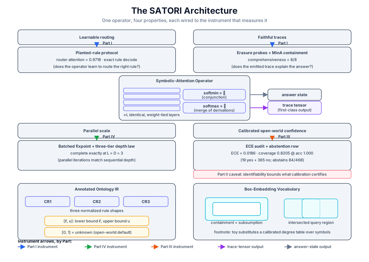Two substrates under one operator, four properties around it, and every claim's arrow terminating at an instrument built by an earlier Part of this volume. Original diagram by the authors, created with AI assistance.

The scorecard, in one table:

property	instrument	built in	committed receipt
learnable routing	planted-rule protocol, exact decode	Part I (extraction fidelity)	$\alpha = 0.9718$ on advises∘advises; decode exact
faithful traces	erasure probes + MinA containment	Part I (justifications, faithfulness)	comprehensiveness 8/8, sufficiency 4/4, trace ⊇ MinA 2/2
parallel scale	batched fixpoint + the truncation law	Part IV (GPU reasoning, work-depth)	100 variants in one stacked pass; complete iff $L \ge D = 3$
calibrated open-world confidence	ECE audit + risk-coverage row	Part III (calibration, abstention); bounded by Part II	ECE $0.0186$; coverage $0.8205$ at answered-accuracy $1.000$

This table, not any single number in it, is the chapter's export. An architecture is a set of claims, and claims-with-instruments is what separates an architecture from a pitch: for every property you intend to advertise, there must exist a measuring device that (a) you did not design alongside the thing it measures, (b) produces a number an assert can guard, and (c) can fail. Every row above could have failed. The router could have concentrated on cites∘advises; the trace could have missed every MinA; recall could have broken soundness on the way up; the abstention policy could have answered wrong. The receipts are worth something precisely because the instruments were capable of returning bad news.

The unsolved part

The four properties are individually evidenced and jointly unexamined. Every receipt above holds one property still while measuring another: the routing experiment runs on crisp features with the annotations off; the calibration audit runs with the rules given, not learned; the truncation table runs with no neural imputation in the loop. The interactions are exactly where a real system would live and exactly where this desk has no numbers. Does training the router degrade the calibration of the degrees flowing through it, the way discriminative fine-tuning routinely degrades calibration elsewhere? Does truncation at $L$ below $D$ bias the traces, systematically recording shallow derivations where the true justification is deep, so that faithfulness passes while the explanation distribution shifts? Does the abstention rule stay sound when the upper bound comes from a learned box rather than a type signature? The ablation matrix that would answer these, four properties on and off in combination, exists as a plan in the project's corpus, not as a result anywhere. And beneath the interactions sits the substrate gap flagged in every section above: the toy gates degrees over given symbols, while the design specifies learned boxes with soft unification, TBox-initialized, disjointness-regularized, transferable. Between those two lies precisely the evidence a desk with thirteen entities cannot produce, and the next chapter's claims matrix is honest about which of its rows wait on it.

Why it matters

This chapter is the volume's argument folded back on itself. Parts I through VI looked like a tour of separate frontier topics: proofs, shortcuts, calibration, scale laws, depth ceilings, benchmarks. Assembled here, they turn out to have been a single sustained act of instrument-building, and the capstone architecture is the first system the full toolkit gets pointed at. For the reader heading into their own research, the portable lesson is the method, not the system. Whatever architecture you build or review next, count its advertised properties, then count its independent instruments; the difference between those two numbers is the amount of pitch in the paper. The four receipts here are toy receipts, and the chapter has said so at every turn; but the shape of the argument, substrates chosen for closure properties, a trace that is the computation rather than a comment on it, one instrument per claim, error directions kept separate for the calibrator, scales to any size. Systems earn trust the way this chapter spends it: one committed number at a time.

Key terms

• Substrate: a representation the operator runs over, chosen for its closure properties rather than its familiarity; SATORI has two, the annotated rule IR and the box vocabulary.
• Annotated ontology IR: the single rule representation (CR1/CR2/CR3 plus chain and copy shapes) into which EL axioms and Horn rules both compile, with a degree slot on every atom.
• Interval annotation $[\ell, u]$: a two-sided degree, lower bound derivable and upper bound possible; the open-world unknown is the full interval $[0,1]$, making abstention a property of the data model.
• Gödel semiring: degrees composed by $\min$ across a derivation's premises and $\max$ across alternative derivations; the kernel computes its temperature-smoothed image and recovers it as $\tau \to 0$.
• Trace tensor: the per-atom record (layer, rule, argmax parents) emitted by the forward pass itself; machine-checkable, and the object faithfulness instruments probe.
• Planted-rule protocol: hide a known rule, train a router over a template space from the rule's answers alone, and require the trained weights to decode back to the hidden rule exactly.
• Router: a softmax distribution $\alpha$ over candidate rule bodies; the routed prediction is the $\alpha$-mixture of per-template kernel messages, trained by the hand-derived gradient $\partial L/\partial w_i = \alpha_i (g_i - \sum_j \alpha_j g_j)$.
• MinA containment: the faithfulness standard for traces, the recorded axiom set must contain a true minimal justification; containment, not equality, because traces need not be minimal.
• Three-tier scaling law: constant depth for the FO-rewritable slice, $O(\log D)$ for the reachability slice, $\Theta(D)$ for the conjunctive core; fixed-$L$ truncation is a theorem-level limit on tier three, not an engineering shortfall.
• Two error directions: truncation loses recall only (sound but incomplete); embedding-side scoring loses precision only (complete but unsound); calibration must audit them separately.
• Claims-with-instruments: the design discipline this chapter exports, no advertised property without an independent, fail-capable measuring device and a committed number.

Where this leads

One chapter remains in the capstone, and it is the accounting. This chapter gave four properties their instruments on the volume's home turf; the project's paper outline freezes a larger matrix, eight claims spanning multi-hop answering, rule learning, faithful traces, GPU scale, calibration, ontology grounding, cross-ontology transfer, and crisp soundness, and not all of them can be honestly tested on thirteen entities. The Eight Claims runs the largest honest subset, prints a table that says toy-verified with this number or cited-only, and why for every row, and treats the refusals as carefully as the receipts, because a claims matrix that cannot say "not shown here" is just a longer pitch.

---

Companion code: examples/frontier/satori_lite.py implements the kernel, the IR compilation from both prior-volume rule sets, the trace recorder, and the truncation law; examples/frontier/satori_eval.py implements the planted-rule router, the erasure and MinA cross-checks, the interval propagation with abstention, and the ECE audit; examples/frontier/gpu_fixpoint.py implements the batched fixpoint. Run each with python3 from examples/frontier/ to reproduce every number in this chapter; every claim is guarded by an assert except the wall-clock timing, which its own output labels as asserted nowhere.