Rule Extraction: Reading Rules Out of Weights

📍 Where we are: Part I · Proofs, Faithfulness, and Trust — Chapter 3. Faithfulness scored an explanation against the model that produced it; this chapter goes one step further and produces the explanation, as an explicit ruleset, then measures how well the ruleset and the model agree.

The previous chapter left us with a discipline: an explanation is worth only as much as its measured agreement with the model's actual mechanism. That discipline invites an obvious escalation. If agreement is the currency, stop scoring explanations that someone else proposed and instead construct the best symbolic surrogate you can, with the agreement score built into the construction. This is rule extraction: given a trained network, produce a set of explicit symbolic rules (a decision tree, a Boolean formula, a list of logical chain rules) that mimics the network, and report how well the mimicry holds. When it works, three prizes arrive at once: you can audit the model by reading the rules, transfer what it learned into a symbolic system that runs without the network, and verify the rules against an independent standard of truth, something no gradient or attention map will ever submit to. When it fails, the failure is a number, not a shrug. This chapter builds both classical styles of extraction on the running academic world, defines the evaluation triad that keeps the enterprise honest, and closes with the exhibit that motivates the next Part: an extraction perfectly faithful to its model and wrong about the world.

The simple version

Imagine a brilliant but wordless craftsman who sorts job applications into yes and no piles, and you want his policy in writing. One approach: hand him thousands of invented applications, record every verdict, and write the shortest rulebook that reproduces his sorting; you never open his head, you only interview him. Another: watch his eyes while he works, note which lines of the form he actually reads, and transcribe those habits into rules. Either way you end with a rulebook and one crucial number: on how many applications does the rulebook match the man? And one trap waits at the end: if the craftsman secretly sorts by postcode, a perfect rulebook will say "sort by postcode", in writing, faithfully. The rulebook tells you what he does. It cannot tell you whether what he does is right.

What this chapter covers

• From scoring to producing: why extraction is faithfulness made constructive, and the three payoffs (audit, transfer, verification) that made the field want it from the early 1990s onward.
• The classical taxonomy: pedagogical methods that query the network as a black box, decompositional methods that read structure out of the weights, and the eclectic middle; what each assumes, and the fidelity metric defined once for all of them.
• Pedagogical extraction done exactly: a seeded multilayer perceptron trained on a hidden Boolean formula, interrogated by membership queries over all sixteen inputs, distilled into a decision tree, minimized to prime implicants, and recovered exactly, with every step asserted in committed code.
• Decompositional extraction on live machinery: Volume 4's Neural-LP head re-imported and retrained bit for bit, its attention unrolled into chain rules with confidences, and the confidence cutoff swept from permissive to fatal.
• The evaluation triad: fidelity (does the ruleset agree with the model?), soundness (do its answers hold in the symbolic closure?), completeness (does it recover all closure answers?), three different questions that one committed table separates cleanly.
• The wrongness exhibit: a network trained on biased data, extracted faithfully, reporting a spurious rule with perfect fidelity; the precise sense in which extraction is a microscope and not a certifier.

From scoring explanations to producing them

The faithfulness chapter treated the explanation as given and asked whether it tracked the model. Extraction inverts the workflow: the explanation is the output, and tracking the model is the objective. This is an old ambition. The survey that organized the field in the mid-1990s catalogued motivations that still hold: extracted rules make a trained network inspectable by people who must sign off on it, portable into systems that cannot run the network, and checkable against domain knowledge the network never saw [1]. The same era built the full round trip: encode what you already know as a network (insertion), train it on data (refinement), and read the improved theory back out (extraction), so that the network becomes a theory reviser rather than an oracle; KBANN (Knowledge-Based Artificial Neural Networks) made that loop concrete, and it returns later in this chapter. One thing did not change from the previous chapter: the manufactured ruleset earns nothing until its agreement with the model is measured, on stated inputs, with a stated metric. Extraction without that measurement is just a second model with better typography.

The taxonomy, and fidelity defined once

The classical taxonomy sorts extraction algorithms by what they are allowed to see [1]. A pedagogical method treats the network as a closed black box: it may pose inputs and observe outputs, nothing more, and it fits a symbolic mimic to that input-output behavior, as a teacher learns a student's misconceptions purely from the student's answers. A decompositional method opens the box: it inspects individual weights, units, or attention distributions and translates each internal structure into a rule. An eclectic method mixes the two. The assumptions differ sharply. Pedagogical methods assume only query access, so they apply to any model whatsoever, but they pay in queries over an input space that is usually astronomically large. Decompositional methods assume the architecture keeps rule-shaped structure worth reading (a unit approximating a logical gate, an attention vector approximating a relation choice); when that holds they are cheap and exact, and when it fails there is simply nothing to read.

style	sees	assumes	pays	companion exhibit
pedagogical	inputs and outputs only	query access	query budget grows with the input space	hidden-formula network, all 16 membership queries
decompositional	weights and activations	rule-shaped internal structure	nothing to read when structure is absent	Volume 4's Neural-LP attention, unrolled
eclectic	both	some of each	some of each	(not built; the two poles suffice here)

One metric serves all three, and the survey made it the field's central criterion: fidelity, the agreement rate between the surrogate and the model [1]. Write it once, in full. Let $f$ be the trained model, $R$ the extracted ruleset, and $Q$ a distribution over inputs $x$ (a rule for choosing which inputs to ask about, with what probability). Then

$$\mathrm{fid}(R, f; Q) \;=\; \Pr_{x \sim Q}\big[\, R(x) = f(x) \,\big],$$

read: draw an input $x$ according to $Q$, ask both the ruleset and the model, and report the probability that they answer identically ($\Pr_{x \sim Q}$ decodes as "the probability, when $x$ is sampled from $Q$"). The distribution $Q$ is not a technicality; it is the third argument of the definition. Fidelity is always fidelity on some inputs: a ruleset can agree with the model perfectly on the training distribution and diverge wildly off it, and the number means nothing until $Q$ is stated. Our exhibits make $Q$ explicit and deliberately total: the pedagogical exhibit measures agreement on all sixteen possible inputs (uniform $Q$ over the whole domain, no sampling gap), and the decompositional exhibit measures agreement on the pooled query-answer decisions of the training queries, in a form made precise in the triad section.

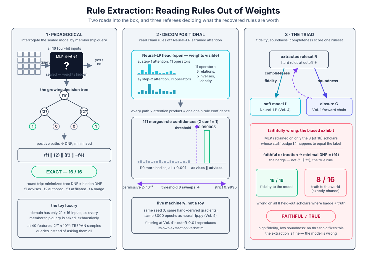Two roads into the box and three referees at the exit: pedagogical extraction interviews the model, decompositional extraction reads its weights, and the fidelity/soundness/completeness triad decides what the recovered rules are actually worth. Original diagram by the authors, created with AI assistance.

Pedagogical extraction, done exactly

The pedagogical exhibit in examples/frontier/rule_extract.py runs the classical pipeline to completion, nothing sampled, nothing approximate. The world has $4$ Boolean features, so an input is a tuple $x = (f_1, f_2, f_3, f_4)$ with each $f_j \in \{0, 1\}$ (read $\in$ as "is one of": each feature is either $0$ or $1$, and the index $j$ ranges over the four features), and the input space has exactly $2^4 = 16$ elements. The features carry the academic world's reading, fixed in the source (rule_extract.py lines 178–190): $f_1$ = advises a student, $f_2$ = authored a paper, $f_3$ = affiliated with a university, $f_4$ = carries a staff badge. The label the network must learn is a hidden disjunctive normal form (DNF) formula, an OR of ANDs of possibly negated features:

$$y \;=\; (f_1 \land f_2) \,\lor\, (f_3 \land \lnot f_4),$$

where $\land$ is AND, $\lor$ is OR, and $\lnot$ is NOT. In the code a conjunction is an implicant tuple with entries $1$ (the feature must hold), $0$ (must fail), or None (not tested), and the hidden formula is the constant HIDDEN_DNF (rule_extract.py line 193). The model is a 4→6→1 multilayer perceptron (MLP): four inputs, six sigmoid hidden units, one sigmoid output, trained by full-batch gradient descent on the mean cross-entropy with every gradient written by hand, exactly Volume 1's machinery (train_mlp, rule_extract.py lines 219–256). Writing $L$ for the mean cross-entropy loss, $z_2$ for the output unit's pre-activation, $p$ for the predicted probability, $y$ for the label, $n$ for the number of training inputs (all $16$ of them here), $\sigma$ for the sigmoid, and $\partial L/\partial z_2$ for the partial derivative of the loss with respect to that pre-activation, the output layer uses the sigmoid-plus-cross-entropy cancellation $\partial L/\partial z_2 = (p - y)/n$ at lines 237–242, and the hidden layer chains through the sigmoid's derivative $\sigma' = \sigma(1 - \sigma)$ at lines 243–248. Seeded at $3$ and run for $3000$ epochs at learning rate $1.0$, its committed loss falls $0.7796 \to 0.6790 \to 0.2961 \to 0.0153 \to 0.0031$ over the snapshot epochs $1, 10, 100, 1000, 3000$, and it fits all sixteen labels. From this point on the weights are sealed. The extraction is not allowed to look at them; it may only ask.

Membership queries and the tree

A membership query poses one input and records the model's hard answer, here $\hat y(x) = 1$ exactly when the output sigmoid clears $1/2$ (mlp_predict, rule_extract.py lines 258–261). Because the domain has sixteen elements, the exhibit queries all of them, so the oracle's behavior is known completely; this is the toy luxury flagged honestly below. On the sixteen answers the extraction grows a decision tree by plain ID3 (Iterative Dichotomiser 3, Quinlan's classic decision-tree learner) [2]: at each node, split on the feature with the greatest information gain. Decode the two quantities. The binary Shannon entropy of a set of labels with positive fraction $p$ is

$$H(p) \;=\; -\,p \log_2 p \;-\; (1 - p)\log_2(1 - p),$$

the average number of bits of surprise per label, zero when the set is pure ($p = 0$ or $p = 1$) and maximal at $p = 1/2$ (entropy, rule_extract.py lines 264–271). The information gain of splitting a node's $n$ examples on feature $f_j$, whose two sides hold $n_0$ and $n_1$ examples, is the entropy removed:

$$\mathrm{IG}(j) \;=\; H(\text{labels}) \;-\; \frac{n_0}{n} H(\text{labels with } f_j = 0) \;-\; \frac{n_1}{n} H(\text{labels with } f_j = 1),$$

with ties broken toward the lowest feature index so the run is deterministic (id3, rule_extract.py lines 273–297). Work the root split by hand, from the committed labels. The hidden formula is true on $7$ of the $16$ inputs ($4$ satisfy $f_1 \land f_2$, another $4$ satisfy $f_3 \land \lnot f_4$, and the input $1110$ satisfies both, so the union has $4 + 4 - 1 = 7$ elements), giving root entropy $H(7/16) = 0.988699$ bits. Each of the four features splits the sixteen inputs into two sides of eight, and each produces one side with $2$ positives of $8$ and one with $5$ of $8$ ($f_1 = 0$, for instance, kills the first disjunct, leaving only the $2$ inputs with $f_3 = 1, f_4 = 0$). So every feature yields the same gain:

$$\mathrm{IG} \;=\; 0.988699 \;-\; \tfrac{8}{16}\, H(2/8) \;-\; \tfrac{8}{16}\, H(5/8) \;=\; 0.988699 - \tfrac{1}{2}(0.811278) - \tfrac{1}{2}(0.954434) \;=\; 0.105843.$$

A four-way tie, resolved to $f_1$ by the deterministic rule. Recursing until every leaf is pure yields a tree of $13$ nodes ($6$ internal, $7$ leaves) that reproduces the oracle on all sixteen queries. On a complete truth table purity is guaranteed: all sixteen inputs are distinct, so in the worst case a path tests all four features, after which its leaf holds exactly one input, and a one-element label set is pure. The recursion must therefore terminate with every leaf pure, so the mimicry is exact by construction (asserted at rule_extract.py lines 424–425).

From tree to minimal DNF

Rules come off the tree mechanically: every root-to-positive-leaf path is one implicant, the conjunction of the tests taken along the path, and the OR of these path implicants fires on exactly the inputs the tree routes to a positive leaf (tree_to_dnf, rule_extract.py lines 304–314). The committed path DNF has three terms and is visibly clumsy, an artifact of the greedy split order rather than of the function. The last step minimizes it with a brute-force Quine–McCluskey [3] pass over all $3^4 = 81$ candidate implicants, each feature independently tested-true, tested-false, or untested (minimize_dnf, rule_extract.py lines 317–345). Three definitions do the work. A candidate is an implicant of the target function when every input it covers has label $1$. An implicant is prime when dropping any single literal breaks that property. A prime is essential when some positive input is covered by no other prime, forcing it into every correct cover. Here exactly two primes survive, both essential: the input $1101$ is covered only by $(f_1 \land f_2)$, and $0010$ only by $(f_3 \land \lnot f_4)$, and the module asserts that the essential primes alone already cover every positive input (lines 342–343), so the minimal cover is unique and no search is needed. The committed run:

[4] pedagogical (TREPAN-style): hidden DNF → MLP → membership queries → tree → minimal DNF
    hidden rule   : y = (f1 ∧ f2) ∨ (f3 ∧ ¬f4)
    MLP 4→6→1 (lr=1.0, seed 3), CE loss: [1] 0.7796  [10] 0.6790  [100] 0.2961  [1000] 0.0153  [3000] 0.0031;  fits 16/16
    ID3 tree on all 16 membership queries: 13 nodes, mimics the oracle 16/16
    tree path DNF : (¬f1 ∧ f3 ∧ ¬f4) ∨ (f1 ∧ ¬f2 ∧ f3 ∧ ¬f4) ∨ (f1 ∧ f2)
    minimized     : (f1 ∧ f2) ∨ (f3 ∧ ¬f4)   (2 prime implicants, all essential)
    round trip    : minimal DNF == hidden DNF — the extraction is EXACT

The recovered formula is the hidden formula, implicant for implicant, and agrees with the model on $16/16$ inputs; both facts are asserts, not observations (rule_extract.py lines 428–431; the model-agreement half routes through the assert at line 421 that the oracle equals the hidden labels). Fidelity is $1.0$ on the entire domain, the strongest statement extraction can ever make.

Now the honesty. Exhaustive querying works because $2^4 = 16$; at forty features the domain has $2^{40}$ elements, roughly $10^{12}$, and complete interrogation is over. TREPAN is the classical answer to that wall [4]: it samples membership queries from a model of the input distribution, conditioned on the constraints along each tree path, so deep nodes still receive enough queries to split reliably; it grows the tree best-first, expanding next the node whose expansion most improves fidelity; and it uses m-of-n split tests (a node test that fires when at least $m$ of its $n$ listed conditions hold) to keep the tree compact. The design principle is the fidelity definition read as an algorithm: spend the query budget where $Q$ puts mass and where disagreement still lives. Our exhibit keeps the pipeline and deletes the budget, which is exactly what a sixteen-element domain permits and nothing larger does. The pedagogical loop also closes a much older circle: KBANN inserted a hand-written domain theory into a network as its initial weights and refined the network on data [5]; its companion extraction paper then read a corrected theory back out and measured it outperforming the one that went in [6]. Extraction there was not an audit but the return path of a round trip in which the network served as a theory reviser, and that round trip remains the historical benchmark for the ambition of neuro-symbolic integration.

Decompositional extraction on live machinery

The second exhibit opens the box, and the box is real: Volume 4's Neural-LP (Neural Logic Programming) head, imported from examples/integration/neural_lp.py and retrained bit for bit inside this module (same seed $0$, same hand-derived gradients, same $3000$ epochs; train_soft_model, rule_extract.py lines 93–103). Recall its anatomy in one paragraph. Every relation of the academic knowledge graph is a TensorLog operator, a $13 \times 13$ adjacency matrix $M_k$ over the $13$ entities whose entry $(h, t)$ is $1$ exactly when the edge $(h, k, t)$ is in the training graph; the operator vocabulary has $K = 11$ entries, the $5$ relations, their $5$ inverses, and the identity. The head answers grandAdvisor(x, ?) by $T = 2$ reasoning steps, each a softmax attention $a_t$ over the operators applied to a softmax attention over the memory of previous states, trained on the atoms Volume 1's forward chainer derives from the same edges [7]. The committed retraining reproduces Volume 4's numbers exactly: loss $13.7083$ at epoch 1 down to $0.0020$ at epoch 3000, and the model's soft answer sets (entities whose score clears the answer cutoff $0.1$) match the symbolic closure, alice → carol and bob → erin.

Extraction is the paper's Algorithm 1: every path through the two-step computation graph is one chain rule, and its confidence is the product of the attention weights along the path [7]. The module unrolls without the reference implementation's confidence cutoff (the paper itself prescribes none; the released repository filters at --rule_thr, default $0.01$, the cutoff Volume 4 adopted), so the cutoff itself becomes the experiment (unroll_rules, rule_extract.py lines 106–133):

    add(float(b3[0]), ())
    for k in range(nlp.K):
        add(float(b3[1] * a1[k]), (nlp.OP_NAMES[k],))
        add(float(b3[2] * b2[0] * a2[k]), (nlp.OP_NAMES[k],))
    for k1 in range(nlp.K):
        for k2 in range(nlp.K):
            add(float(b3[2] * b2[1] * a1[k1] * a2[k2]),
                (nlp.OP_NAMES[k1], nlp.OP_NAMES[k2]))

Here $a_1, a_2$ are the two operator attentions and $b_2, b_3$ the memory attentions, each a softmax and therefore a probability vector. The step-$t$ memory attention has one entry per state available to attend over, the initial one-hot state plus each previous step's result: $b_2 = (b_2[0], b_2[1])$ chooses between the initial state and step 1's output, and $b_3$'s three entries choose among the initial state (reading it out directly yields the empty body, the identity chain), step 1's output, and step 2's output. That softmax fact yields a clean conservation law: summing the confidence over all paths, using $\sum_k a_1[k] = \sum_k a_2[k] = 1$ (the summation adds one term per operator index $k$),

$$\sum_{\text{paths}} \mathrm{conf} = b_3[0] + b_3[1]\!\sum_k a_1[k] + b_3[2]\, b_2[0]\!\sum_k a_2[k] + b_3[2]\, b_2[1] \Big(\sum_{k_1} a_1[k_1]\Big)\Big(\sum_{k_2} a_2[k_2]\Big) = b_3[0] + b_3[1] + b_3[2]\big(b_2[0] + b_2[1]\big) = 1,$$

since $b_2$ and $b_3$ are themselves probability vectors. The unrolled confidences form a probability distribution over rule bodies, asserted to machine precision (rule_extract.py line 385), and filtering the full list at Volume 4's cutoff $0.01$ must reproduce Volume 4's own extraction verbatim, also asserted (lines 387–388). After merging identical bodies (identity hops dropped), the committed read-off:

[2] decompositional read-off (Neural LP Algorithm 1, NO cutoff): 111 merged bodies, Σ conf = 1
    0.999005  grandAdvisor(X,Y) ← advises(X,Z1) ∧ advises(Z1,Y)
    0.000339  grandAdvisor(X,Y) ← advises(X,Y)
    0.000111  grandAdvisor(X,X) ← ⊤   (the identity chain)
    0.000032  grandAdvisor(X,Y) ← inv_advises(X,Z1) ∧ advises(Z1,Y)
    ... and 107 more, none above 0.000032; filtered at Volume 4's cutoff 0.01 == nlp.extract_rules

One rule holds $99.9\%$ of the attention mass, and it is Volume 1's rule: a grand-advisor is an advisor's advisor. The other $110$ bodies share a tenth of a percent. This is decompositional extraction under the best possible conditions: an architecture whose internal structure is a distribution over rule bodies, trained to near-certainty on a task with one true rule. What a threshold does to this list is the interesting question, and it needs the triad.

The triad: three referees, three questions

A thresholded ruleset can be judged against two different authorities, and the judgments must not be blurred. The module fixes the objects once (rule_extract.py lines 80–82). The query set is the two training queries, alice and bob. For a cutoff $\theta$ (the Greek letter theta, the confidence threshold), the hard answer set $H$ pools every pair $(x, y)$ such that some rule with confidence at least $\theta$, applied purely symbolically from $x$ over the training edges (set-valued hops, no floats; Volume 4's apply_rule, neural_lp.py lines 296–313), reaches $y$. The soft answer set $S$ pools the model's own thresholded answers, $y$ with score $p_y \ge 0.1$. The closure $C$ is Volume 1's forward-chained ground truth over the same edges, exactly two pairs here, (alice, carol) and (bob, erin). Three ratios, three questions (triad_at, rule_extract.py lines 155–173):

$$\mathrm{fidelity} = \frac{\lvert H \cap S \rvert}{\lvert H \cup S \rvert}, \qquad \mathrm{soundness} = \frac{\lvert H \cap C \rvert}{\lvert H \rvert}, \qquad \mathrm{completeness} = \frac{\lvert H \cap C \rvert}{\lvert C \rvert},$$

where $\lvert \cdot \rvert$ counts a set's elements, $\cap$ is intersection and $\cup$ is union; the fidelity ratio is the Jaccard index, intersection size over union size, and soundness is left undefined when $H$ is empty (there is nothing to be sound about). Fidelity asks: do the rules answer like the model? Soundness: of what the rules answer, how much does the closure confirm? Completeness: how much of the closure do the rules recover? The first is the extraction community's criterion; the last two are Volume 2's logician asking her two eternal questions of any derivation system.

The fidelity ratio deserves one derivation, because the obvious alternative is a trap. Why Jaccard agreement over pooled positive pairs rather than plain per-decision agreement? There are $2 \times 13 = 26$ (query, entity) decisions in play, and the true answers are only $2$ of them. An empty ruleset disagrees with the soft model only on the model's $2$ positives, so per-decision agreement hands it $24/26 = 0.923$, a sterling score for a surrogate that says nothing: class imbalance masquerading as fidelity (rule_extract.py lines 162–164). The Jaccard form scores the empty ruleset $0/2 = 0$, which is what it earned. The sweep grid is chosen around the structure of the unrolled list (rule_extract.py lines 83–86): below the weakest surviving path family ($2 \times 10^{-5}$), between the path families ($10^{-4}$, $5 \times 10^{-4}$), at the reference implementation's default cutoff ($0.01$), and past the top rule's confidence $0.999005$ (the cutoff $0.9995$). The committed table:

[3] the fidelity triad vs the cutoff — compactness against agreement
    cutoff    #rules  #answers  fidelity  soundness  completeness
    2e-05        21         9     0.222      0.222         1.000
    0.0001        3         6     0.333      0.333         1.000
    0.0005        1         2     1.000      1.000         1.000
    0.01          1         2     1.000      1.000         1.000
    0.5           1         2     1.000      1.000         1.000
    0.9995        0         0     0.000         --         0.000
    too permissive drowns the 2 sound answers among 9; too strict (0.9995 > top conf 0.999005) keeps none

Read it row by row. At $2 \times 10^{-5}$, twenty-one rules survive and jointly answer $9$ pairs; the $2$ true answers are among them (completeness $1.000$) but drown in $7$ spurious ones, so fidelity and soundness both fall to $2/9 = 0.222$. At $10^{-4}$, three rules answer $6$ pairs: $2/6 = 0.333$. From $5 \times 10^{-4}$ through $0.5$, three decades of threshold, exactly one rule survives, advises∘advises, and the triad is perfect. At $0.9995$ the threshold passes the top rule's own confidence and the ruleset is empty: fidelity $0$, completeness $0$, soundness undefined. Both ends collapse, and the run asserts the whole shape: monotone rule counts, the drowning at the permissive end, the perfect band, the empty strict end (rule_extract.py lines 399–410).

The honest reading of the trade: compaction was nearly free here because the trained attention had concentrated $99.9\%$ of its mass on one body, so the last rule standing was the right one and it died only when the threshold exceeded $0.999$. Where attention is diffuse, several bodies sharing the mass of one true rule (the entangled rank-1 heads of Volume 4's DRUM exhibit are the canonical case), each fragment's confidence is low, thresholds bite early, and fidelity falls as the ruleset compacts, fragment by fragment. Compactness and fidelity are in tension exactly to the degree that the model's internal structure fails to be rule-shaped.

The triad's value is diagnostic, because its three numbers fail in distinguishable patterns:

pattern	committed instance	diagnosis
high fidelity, high soundness, high completeness	the $5 \times 10^{-4}$ to $0.5$ band	the model is right and the rules capture it; the extraction is a certificate of both
low fidelity, low soundness, completeness $1.0$	the $2 \times 10^{-5}$ row	an over-generating surrogate: the truth is in there, buried; raise the threshold
high soundness, low completeness	(not reached on this head; one rule already covers $C$)	a cautious partial theory: everything it says checks out, but it is silent on part of the closure
high fidelity, low soundness	the biased exhibit, next	the extraction is fine and the model is wrong; no threshold will fix it

The first three patterns are about the extraction. The last one is about the world, and it is the chapter's deepest point.

Faithfully wrong: the exhibit that earns the next chapter

Retrain the same 4→6→1 MLP, same seed, same code path, on a biased sample. The world's true rule, Volume 2's professorship axiom in Boolean dress, is $y = f_1 \land f_2$: a professor advises and has authored. But the sample contains only the $8$ scholars (of $16$) whose staff badge agrees with their true status: every sampled professor carries a badge, every sampled non-professor lacks one (biased_sample, rule_extract.py lines 353–363; the kept inputs are numbers $0, 2, 4, 6, 8, 10, 13, 15$). On this sample the badge alone is a perfect predictor, and it is simpler than the true rule: one feature instead of two. Gradient descent takes the cheap path, fits its sample $8/8$ with a final cross-entropy of $0.0004$, and the sealed box goes through the same extraction pipeline: membership queries on all sixteen inputs, ID3, minimization. The committed result:

[5] the honest exhibit: a faithful extraction of a WRONG model
    world rule    : professor ⟺ (f1 ∧ f2)   [f1 advises, f2 authored]
    biased sample : only the 8 scholars whose staff badge f4 equals the label are observed
    biased MLP    : fits its sample 8/8; CE loss [3000] 0.0004
    extraction    : tree 3 nodes → minimal DNF (f4)   [the badge, not the professorship]
    fidelity-to-model 16/16   truth-to-world 8/16 (exactly chance)
    wrong on all 8 held-out scholars where badge and truth part ways — faithfully wrong

The tree is three nodes, a single split on $f_4$, and the minimal DNF is the single literal $(f_4)$: carries a badge. The extraction is flawless as an extraction: it agrees with the model on all sixteen inputs, and the run asserts both the perfect fidelity and the fact that every extracted implicant hinges on the badge, a feature the world's rule never mentions (rule_extract.py lines 446–451). And it is wrong about the world on exactly the $8$ held-out scholars where badge and truth part ways: $8/16$ overall, precisely chance, asserted input by input (lines 453–455). The extraction did not fail. It succeeded, and its success is the report: this model classifies by the badge.

State the moral with care, because both halves matter. Extraction is a microscope: it makes the model's decision policy visible in a vocabulary a human or a reasoner can inspect, and a high-fidelity extraction of a spurious policy is the microscope working, not breaking. What extraction is not is a certifier: fidelity is agreement with the model, and no function of the model alone can certify the model against the world. Certification needs an authority the model did not train on: a symbolic oracle (the triad's soundness leg did exactly this, checking $H$ against Volume 1's closure), or held-out interventions, inputs deliberately constructed where the suspected shortcut and the truth disagree, which is precisely what the eight held-out scholars are. The biased model is this volume's first sighting of a phenomenon important enough to own the next Part: a model right on everything it was trained on, for a reason that is wrong, and systematically so.

Where extraction lives now

The classical pipeline survives, but its center of gravity moved into the architectures themselves. Differentiable rule learners ship extraction as a feature, not a post-hoc rescue: Neural-LP's training loop ends by writing out its rules with confidences, the exact Algorithm 1 unrolled above [7], and DRUM reads confidence-carrying rules off its low-rank attention chains the same way, presented as a confidence-sorted list, the low-rank structure existing precisely so that independent rules do not entangle in the read-off [8]. The field's own caveat travels with the feature: a rule read off soft attention is proof-shaped, not a proof. Its body was scored by products of continuous weights over soft adjacency masses, and nothing in that arithmetic guarantees that the discrete rule, applied as logic, derives what the model derived. The repair is re-verification, and both volumes practice it: Volume 4 replayed the extracted top rule purely symbolically, asserting it reproduces every training answer and transfers to the held-out edge (neural_lp.py lines 296–313 and 497–502), and this chapter's soundness leg re-verifies every surviving rule against the closure at every threshold. KBANN remains the benchmark of what the loop is for: rules in, refinement by gradient, better rules out, each leg measured [5][6]. Extraction at its best is not an autopsy; it is the read-out half of a conversation between a theory and its data.

The unsolved part

Both of this chapter's successes leaned on structure. The pedagogical exhibit had a sixteen-element domain, so fidelity could be measured everywhere; the decompositional exhibit had an architecture whose parameters literally are a distribution over rule bodies. Neither crutch exists for a large distributed model. A transformer's weights offer no per-rule anatomy to unroll: whatever regularities it learned are smeared across attention heads and feed-forward layers in superposition, and decompositional extraction has no object to decompose. Pedagogical extraction still applies in principle, needing only query access, but its metric quietly breaks: for open-ended inputs there is no canonical $Q$, no way to enumerate, and no guarantee that agreement measured on today's $Q$ survives tomorrow's distribution shift; a surrogate faithful on the benchmark can be arbitrarily unfaithful one paraphrase away. Underneath both problems sits the granularity question this Part keeps meeting: rules over which vocabulary? Our exhibits were handed their atoms ($f_1$ through $f_4$, the eleven operators), and the extraction only had to arrange them. When the model's internal features align with no human predicate, there may be no vocabulary in which a compact, faithful ruleset exists at all. The honest summary: extraction works where architectures kept structure, one more argument, banked for Part VII, for building the structure in rather than hoping to find it afterward.

Why it matters

This chapter turns the volume's trust question into an engineering loop with a scoreboard. Faithfulness gave us the criterion; extraction gives a constructive procedure that optimizes it, and the triad prices the product against each authority separately: the model (fidelity), the logic (soundness), and the logic's full extent (completeness). For the series arc, the two exhibits are the two halves of the neuro-symbolic bargain made checkable: the pedagogical round trip recovers Volume 1's Boolean world from a gradient-trained network, and the decompositional read-off cashes out Volume 4's central claim that a differentiable architecture can contain its own symbolic theory. For your own research the portable lesson is the biased exhibit: whenever you extract, publish the referee along with the fidelity number, because a surrogate can only ever be as truthful as the model it mimics, and that gap is measurable only against ground truth the model never controlled.

Key terms

• Rule extraction: producing an explicit symbolic surrogate (tree, DNF, chain rules) for a trained network, together with a measured agreement between the two.
• Pedagogical / decompositional / eclectic: the classical taxonomy by access: query the model as a black box; read structure out of its weights; or mix the two.
• Membership query: one input posed to the model as an oracle, its hard answer recorded as a training label for the surrogate.
• Fidelity: the agreement rate between surrogate and model over a stated query distribution $Q$; always fidelity on some inputs, never in the abstract.
• Soundness / completeness (of a ruleset): the fraction of the ruleset's answers confirmed by the symbolic closure, and the fraction of the closure's answers the ruleset recovers.
• Implicant, prime implicant, essential prime implicant: a conjunction covering only positive inputs; one that can drop no literal; one that some positive input needs uniquely. The vocabulary of DNF minimization.
• Chain rule (in rule learning): a rule whose body is a sequence of relations composed along a path, read off attention products with a confidence in Neural-LP-style extraction.
• Proof-shaped, not a proof: the status of a rule read off soft attention before symbolic re-verification; the soundness leg of the triad is the re-verification.
• Faithfully wrong: a high-fidelity extraction of a model whose learned policy is spurious; the extraction succeeds precisely by reporting the wrong rule.

Where this leads

The biased MLP was caught only because we possessed the world's true rule and eight held-out scholars where the shortcut and the truth disagree. The next chapter asks what happens when we are not so lucky: when a model, and in particular a neuro-symbolic model whose concepts are supposed to mean something, achieves the right answers through systematically wrong internal rules, and the training signal is provably unable to notice. That phenomenon has a name, a counting theory, and a benchmark suite, and it occupies Reasoning Shortcuts.

---

Companion code: examples/frontier/rule_extract.py implements both exhibits and the triad: the cutoff-free unrolling of Volume 4's Neural-LP head with the threshold sweep, the membership-query distillation (MLP, ID3, Quine–McCluskey) with its exact round trip, and the biased-data extraction, every claim guarded by an assert. Run python3 examples/frontier/rule_extract.py to reproduce every number in this chapter; the run is deterministic, and the imported soft model retrains bit for bit from examples/integration/neural_lp.py.