Measuring Shortcuts: rsbench and Concept Quality

📍 Where we are: Part II · Identifiability and Reasoning Shortcuts — Chapter 6. Identifiability proved that label metrics are blind to every symmetry of the knowledge; this chapter builds the instrument that measures what labels cannot see.

Part II has delivered a negative result in two installments. Reasoning Shortcuts counted the label-perfect relabelings of a model's concepts: sixteen admissible maps on the XOR (exclusive-or) task, fifteen of them wrong, and thirty-two, thirty-one wrong, once one training combination goes missing. Identifiability explained why every one of them is invisible where training looks: the bijective relabelings that commute with the knowledge on every state form a group, and no label metric, on any test set, at any size, can distinguish two models that differ by such a relabeling; the remaining admissible maps are equally invisible on the observed support. A theorem that says "your favorite metric cannot see the failure" forces a constructive question: what would see it? The answer is not a cleverer statistic computed from the same labels; the theorem forbids that. The answer is a change in what the benchmark itself ships. If concepts are to be scored, the benchmark must carry concept-level ground truth; if the danger is to be known in advance, the benchmark must count its own optima; if the danger is to be dialed up and down, the observed support must be a knob. This chapter derives that requirements list from the theory, introduces the reference suite that institutionalizes it, and then works through the companion's desk-scale rebuild, ending in the committed head-to-head that is the chapter's spine: two models from the same initialization, indistinguishable at label accuracy 1.000, separated by every concept metric in the panel.

The simple version

Imagine grading a mathematics exam two ways. The cheap way scores only the final answer: two students both write "42", both get full marks. The expensive way collects the worked solution and grades every step against a rubric. Now the two students separate: one derived 42 by correct algebra; the other memorized the answer key and, when you read the work, wrote the same meaningless step on every line. Notice what the expensive grading required: the graders had to know the correct work in advance, not just the correct answer. A shortcut-aware benchmark is the expensive exam. The final answer is the label, the worked solution is the model's concepts, the rubric is concept-level ground truth that only the benchmark's designer can supply, the student who reuses one step everywhere is what this chapter calls collapse, and the student who is supremely confident while writing nonsense is what the calibration metric catches. This chapter is about building that exam so the grading is automatic.

What this chapter covers

• The requirements list, derived before the product: what Part II's theory forces a shortcut-aware benchmark to ship, item by item, and the reference suite (generators, an optima counter, a concept-metric panel) that ships exactly that list.
• The generator, quoted: seeded parity and CNF (conjunctive normal form) tasks over latent bits, with a support-bias knob, distractor dimensions, and gold concepts on every split, each contract asserted rather than assumed.
• The counter and its #SAT reduction: the shortcut count as a factored product derived step by step, the closed form for parity, the real suite's reduction to propositional model counting with an approximate counter at scale, and the toy's exhaustive enumeration serving as that machinery's oracle at small size.
• The metric panel, each metric derived then implemented: label accuracy against concept accuracy, macro-averaged concept F1, concept collapse (the paper's count of never-predicted states, refined in the companion to one minus a normalized entropy), and a ten-bin expected calibration error on the concept heads.
• The committed head-to-head: a collapsing shortcut and its concept-supervised twin from the same initialization, read column by column, with every directional claim guarded by an assert.
• Out-of-distribution evaluation as the cheap alarm: why a shortcut fitted to the support must fail off it, how the committed counts quantify exactly how often, and why the rescue of label-only evaluation is only partial.
• The instrument designer's checklist: the four principles this suite satisfies and the later benchmark chapters of this volume will apply to reasoning benchmarks broadly.

The benchmark designer's corner: what theory forces the instrument to ship

Put yourself in the designer's chair and take Part II's results as constraints. Recall the objects: a task has a set $\mathcal{G}$ of ground-truth concept states (for $k$ binary concepts, the $2^k$ joint bit-vectors, where $k$ counts the latent concepts), a fixed piece of knowledge $\mathsf{K}$ acting as a label map $\beta_{\mathsf{K}} : \mathcal{G} \to \{0, 1\}$ that sends each concept state to its label, and an observed support, the subset of $\mathcal{G}$ that training data actually visits. A reasoning shortcut (RS) is an unintended optimum: a relabeling $\alpha : \mathcal{G} \to \mathcal{G}$, different from the identity, with $\beta_{\mathsf{K}}(\alpha(g)) = \beta_{\mathsf{K}}(g)$ for every $g$ in the support, so that a model whose concepts mean $\alpha(g)$ when the world is in state $g$ makes every label come out right. Five design requirements follow, each from a specific result:

Part II result	what it forces the benchmark to ship	companion implementation
Concept accuracy is undefined without a reference; labels cannot substitute for one	gold concepts $g$ attached to every example, in every split	make_task returns $(X, G, Y)$ triples (inputs, gold concepts, labels) for train, test, and out-of-distribution splits (rsbench_lite.py lines 123–159)
Admissibility is a property of $\beta_{\mathsf{K}}$; without the knowledge, "wrong concepts" has no meaning	the knowledge $\mathsf{K}$, known and fixed, published with the task	the label function is $k$-bit XOR or a seeded, printed CNF (lines 83–110)
Shrinking the support strictly enlarges the optimum set	the support as a controllable knob, not an accident of collection	support_frac plus a seeded permutation of $\mathcal{G}$ (lines 137–141)
The number of optima is a task property, computable before any training	a counter for the label-preserving relabelings	count_rs plus its brute-force oracle (lines 164–206); certified at lines 331–341 and 357–361
No label metric separates models that differ by a symmetry	concept-level metrics, scored against the gold concepts	AccC, macro F1(C), collapse Cls(C), and concept ECE, the expected calibration error (lines 213–268)

Only after the requirements are on the table does it make sense to name the product. The reference suite, rsbench, ships exactly this list at research scale [1]: a family of task generators whose ground-truth concepts and knowledge are known by construction (the suite calls the generator layer rssgen), a training-free verifier that counts the label-preserving relabelings a task admits (count-rss), and an evaluation layer that scores concepts separately from labels (rsseval). It is the direct operationalization of the theory the previous two chapters developed, by the same research line [2]: the count the verifier computes is precisely the $N_{\mathrm{opt}}$ of the shortcut-counting theorem, and the metric panel exists because that theorem's conclusion, that label likelihood does not identify concept semantics, closes every cheaper route. The companion module rsbench_lite.py rebuilds all three layers at desk scale, on the same two-bit XOR task the previous chapters trained, so that every number in this chapter is a committed, asserted output rather than a citation.

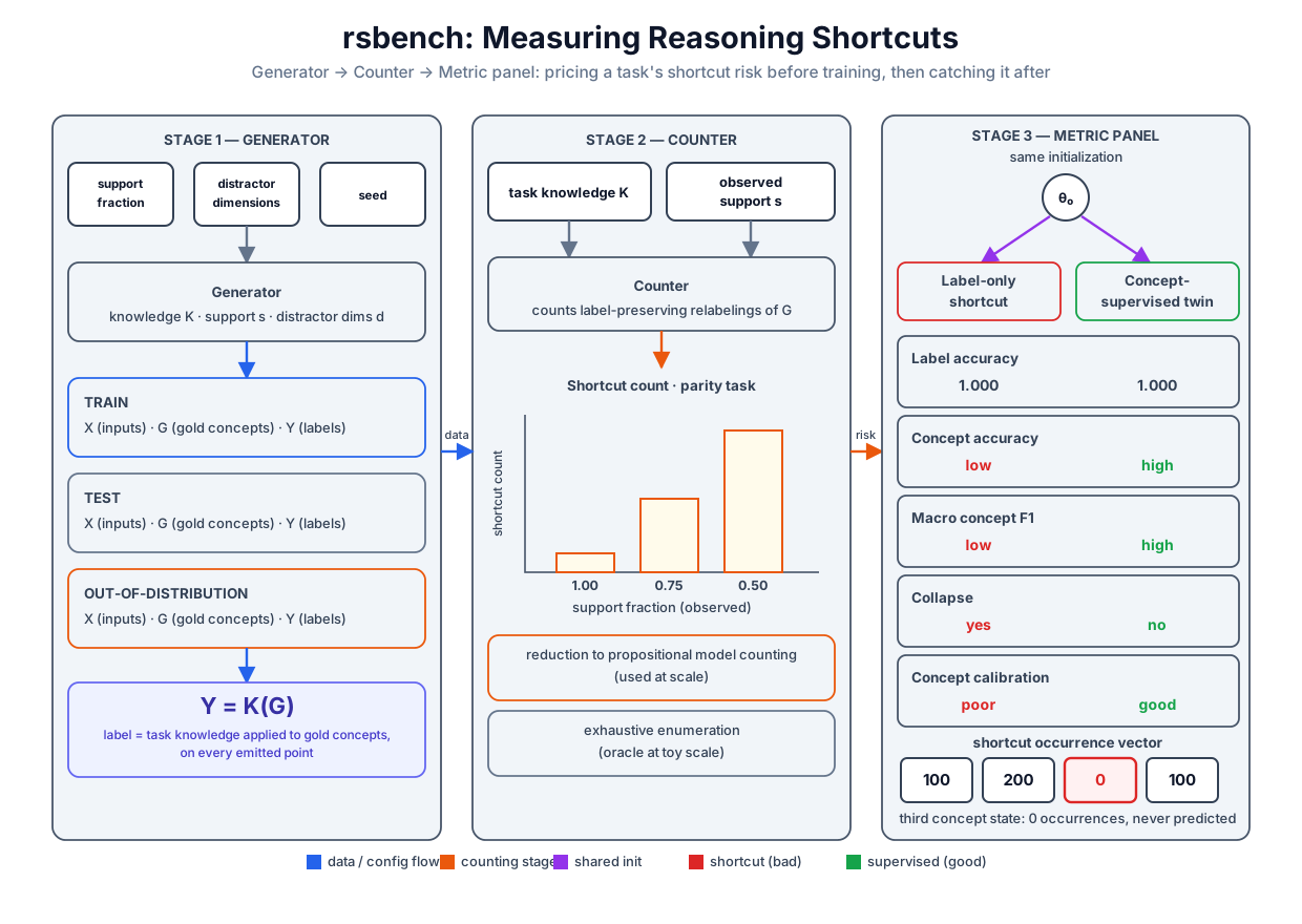The instrument in three stages: a generator that ships gold concepts, a counter that prices the task's danger before training, and a metric panel that separates what label accuracy cannot. Original diagram by the authors, created with AI assistance.

The generator: gold concepts by construction

A generator can guarantee what a collected dataset can only hope for: that every example's concepts are known, because the concepts were sampled first and the observation was rendered from them. The companion's make_task follows the shape of the suite's logic-task family (in rsbench, the MNLogic generator [1]): sample a concept state $g$, a vector of $k$ bits; compute the label $y = \beta_{\mathsf{K}}(g)$ from the knowledge, never from the input; then render the input $x$ from $g$. The rendering places coordinate $j$ of the input at $2g_j - 1$, which maps the bit values 0 and 1 to the corners $-1$ and $+1$, and adds Gaussian scatter of scale $\sigma = 0.25$ (the same corner-cluster geometry the previous chapters used, imported rather than retyped). After the $k$ concept-bearing coordinates come n_distractors pure-noise coordinates that carry no concept at all (rsbench_lite.py lines 147–151):

        # x_concept = (2g − 1) + σ·ε ; x_distractor ~ N(0, 1), concept-free.
        x = np.hstack([
            (2.0 * g - 1.0) + NOISE * rng.standard_normal((len(g), k)),
            rng.standard_normal((len(g), n_distractors))])
        y = np.array([label_fn(tuple(row)) for row in g], dtype=int)

The support knob works by permutation: a seeded shuffle of the $2^k$ concept states keeps the first $\max(1, \mathrm{round}(\text{support\_frac} \cdot 2^k))$ as the observed support; train and test draw balanced samples from the support only, and a third split, ood (out-of-distribution), covers exactly the unobserved states (lines 137–159). Every promise is asserted, not documented: the harness checks generative consistency ($y = \beta_{\mathsf{K}}(g)$ on every emitted point), checks that the realized train support equals the requested one, that the ood split covers exactly the complement, that each concept coordinate actually carries its bit, and that no distractor leaks label signal (lines 303–325). The committed run:

[1] rssgen-lite: seeded generator — k-bit XOR / random CNF over latent bits,
      support bias, distractor dims; every split ships its gold concepts g
      demo task: k=2 XOR, full support, 2 distractor dims (20 train / 50 test per world)
      split   points  input dims  worlds seen  y = XOR(g) on every point
      train      80           4           4  holds (asserted)
      test      200           4           4  holds (asserted)
      ood         0           -           0  empty at full support
      concept dims carry their bit:   corr(x_j, g_j) = 0.972, 0.970
      distractors carry no label:  |corr(x_d, y)| = 0.025, 0.098
      support bias 0.5: train sees only {00, 10}; the ood split covers exactly {01, 11}

Read the two correlation lines as the generator's honesty certificate. The concept-bearing coordinates correlate with their bits at 0.972 and 0.970 (the intended semantics is reachable: a model could learn the right concepts from these inputs), while the distractors correlate with the label at 0.025 and 0.098, sampling noise around zero (the wrong semantics is not smuggled in through a side channel). The asserts demand at least 0.9 for the former and at most 0.3 in absolute value for the latter (lines 317–318). The last line is the knob that matters for this chapter: at support_frac=0.5 the task trains on the concept states 00 and 10 only, and ships an ood split covering exactly 01 and 11. This is the move behind the suite's biased dataset variants, where a digit-pair addition task observes only all-even or all-odd digit pairs in training (the MNAdd-EvenOdd variant), never a mixed pair [1]; the next section prices exactly what that bias costs.

Counting the ways to be wrong before training anything

The counter is the requirement most benchmarks skip and the one this suite is named for. The quantity comes from the shortcut-counting theorem of the previous chapters [2], restated precisely. Let $\mathcal{G}$ be the set of concept states, $s \subseteq \mathcal{G}$ the observed support ($\subseteq$ reads "is a subset of"), and $\beta_{\mathsf{K}}$ the label map. The number of deterministic optima is the number of relabelings that preserve every observed label:

$$N_{\mathrm{opt}} \;=\; \big\lvert \{\, \alpha : \mathcal{G} \to \mathcal{G} \;\text{ such that }\; \beta_{\mathsf{K}}(\alpha(g)) = \beta_{\mathsf{K}}(g) \text{ for all } g \in s \,\} \big\rvert,$$

where $\lvert \cdot \rvert$ counts the elements of a set and $\in$ reads "is a member of". The identity map is always in the set (it changes nothing, so it preserves every label), so the number of reasoning shortcuts is $N_{\mathrm{opt}} - 1$. The proof that these maps exhaust the deterministic optima of the label likelihood belongs to the source [2] and is beyond this volume; what the companion owns is the computation of $N_{\mathrm{opt}}$, and that computation has a structure worth deriving in full.

The defining condition constrains each image $\alpha(g)$ separately: the clause for $g$ mentions $\alpha(g)$ and no other value of $\alpha$. A function $\alpha$ is one independent choice of image per state, so the count of functions satisfying per-state constraints is the product, over states, of the number of allowed images for that state. Split the states into observed and unobserved. If $g \in s$, the image must land in $g$'s label class, the set of states carrying the same label, $\{ c \in \mathcal{G} : \beta_{\mathsf{K}}(c) = \beta_{\mathsf{K}}(g) \}$. If $g \notin s$ ($\notin$ reads "is not a member of"), the condition says nothing, and the image may be any of the $\lvert \mathcal{G} \rvert$ states. Therefore

$$N_{\mathrm{opt}} \;=\; \prod_{g \in s} \big\lvert \{ c \in \mathcal{G} : \beta_{\mathsf{K}}(c) = \beta_{\mathsf{K}}(g) \} \big\rvert \;\cdot\; \prod_{g \notin s} \lvert \mathcal{G} \rvert,$$

where $\prod$ multiplies one factor per state. This factorization is the same structural move the suite's theory uses to collapse otherwise astronomical counts, and it is the entire body of the companion's counter (rsbench_lite.py lines 182–192):

    worlds = all_worlds(k)
    supp = set(support)
    n = 1
    for g in worlds:
        if g in supp:
            # observed: α(g) must land in g's label class, enumerated.
            n *= sum(1 for c in worlds if label_fn(c) == label_fn(g))
        else:
            # unobserved: α(g) is unconstrained — any of the 2^k worlds.
            n *= len(worlds)
    return n

For $k$-bit parity the factors have a closed form. Fix the first $k-1$ bits of a state freely, $2^{k-1}$ ways; the last bit is then forced by the parity you want, so each of the two label classes contains exactly $2^{k-1}$ of the $2^k$ states. Substituting into the factorization, with $\lvert s \rvert$ observed states,

$$N_{\mathrm{opt}} \;=\; \big(2^{k-1}\big)^{\lvert s \rvert} \cdot \big(2^{k}\big)^{2^{k} - \lvert s \rvert} \;=\; 2^{(k-1)\lvert s \rvert} \cdot 2^{k\,(2^{k} - \lvert s \rvert)}.$$

Certification, three ways. A counter that is only ever compared to itself proves nothing, so the module certifies count_rs against three independent oracles before printing a single row (lines 331–341): a literal sweep of all $\lvert \mathcal{G} \rvert^{\lvert \mathcal{G} \rvert} = 4^4 = 256$ maps at $k = 2$ (no factorization, no closed form; lines 195–206), run for both label kinds and four different supports; the previous chapters' own enumeration, which found 16 optima at full support and 32 at the biased support; and the parity closed form just derived, asserted for every row of the table below (lines 357–361).

The honest scale note. Exhaustive enumeration dies fast: at $k = 10$ there are $1024^{1024}$ candidate maps, unwritable, and even the factored product needs the label-class sizes, which for an arbitrary knowledge means counting satisfying assignments. The real suite therefore encodes the condition "$\alpha$ preserves every observed label" as a propositional formula in DIMACS CNF format (the standard file format for conjunctive normal form) and hands it to a #SAT solver, a model counter: exact counting for small tasks, and at scale an approximate counter in the ApproxMC family [3], which returns an estimate $\hat{N}$ with the $(\varepsilon, \delta)$ guarantee that $\hat{N}$ lies within a factor $1 + \varepsilon$ of the true count $N$, that is $N / (1+\varepsilon) \le \hat{N} \le (1+\varepsilon) N$, with probability at least $1 - \delta$. The hashing argument behind that guarantee is beyond this volume. What the companion demonstrates instead is the contract: at small $k$, exhaustive enumeration is tractable and computes the exact answer that any such counter, exact or approximate, is promising to approach; the toy is the oracle for the machinery, not a substitute proof of it. The committed table:

      RS count vs support fraction (support read off the generated train split):
      task  k  support  frac    N_opt      reasoning shortcuts (N_opt - 1)
      XOR   2    4/4    1.00        16         15
      XOR   2    3/4    0.75        32         31
      XOR   2    2/4    0.50        64         63
      XOR   3    8/8    1.00    65,536     65,535
      XOR   3    6/8    0.75   262,144    262,143
      XOR   3    4/8    0.50 1,048,576  1,048,575
      CNF   3    8/8    1.00    84,375     84,374
      CNF   3    6/8    0.75   600,000    599,999
      CNF   3    4/8    0.50 2,560,000  2,559,999
      the seeded CNF (k=3): (x1 | x2 | x3) & (x2 | x3 | ~x1) & (~x3 | ~x2 | x1)   (5/8 worlds satisfy)

Work the parity rows by the closed form. At $k = 3$, full support has $\lvert s \rvert = 8$, so $N_{\mathrm{opt}} = 2^{2 \cdot 8} \cdot 2^{3 \cdot 0} = 2^{16} = 65{,}536$. Dropping to six observed states gives $2^{2 \cdot 6} \cdot 2^{3 \cdot 2} = 2^{12+6} = 2^{18} = 262{,}144$, and to four gives $2^{8} \cdot 2^{12} = 2^{20} = 1{,}048{,}576$: every two states removed from the support multiply the optima by four. The CNF rows have no symmetric closed form, but the factorization still reads them off. The printed formula is satisfied by 5 of the 8 states, so its label classes have sizes 5 and 3; at full support $N_{\mathrm{opt}} = 5^5 \cdot 3^3 = 3125 \cdot 27 = 84{,}375$. At six observed states the realized support kept five satisfying states and one falsifying state, giving $5^5 \cdot 3^1 \cdot 8^2 = 3125 \cdot 3 \cdot 64 = 600{,}000$, and at four it kept only satisfying states, giving $5^4 \cdot 8^4 = 625 \cdot 4096 = 2{,}560{,}000$. The module asserts strict monotone growth along every task's row (lines 366–368): shrinking the support never removes an optimum, because dropping a state drops a constraint; and the growth is strict, because a dropped state's factor changes from its label-class size, which is strictly smaller than $\lvert \mathcal{G} \rvert$ whenever both labels are realized (the CNF generator redraws until they are; lines 89–103), to exactly $\lvert \mathcal{G} \rvert$. Fewer observations, more ways to be wrong, now as a certified number a designer can print on the task's datasheet before anyone trains anything.

The metric panel: five ways to score a concept

The counter prices the task; the metrics score the model. The companion's panel implements the suite's evaluation layer from formulas, five numbers per model, each aimed at a distinct failure.

AccY and AccC, the diagnostic gap. Write $\hat{y}_i$ for the model's predicted label on test point $i$ and $\hat{c}_{ij}$ for its predicted value of concept $j$ there, read off as the argmax (the highest-probability value) of concept head $j$'s softmax. Label accuracy AccY is the fraction of test points with $\hat{y}_i = y_i$; concept accuracy AccC is the fraction of (point, concept) pairs with $\hat{c}_{ij} = g_{ij}$, the gold bit (shortcuts.py lines 287–296, reused unchanged; never duplicate an engine). Neither number is novel; the pair is the instrument. Part II's theory says AccY can sit at 1.000 while the concepts are systematically wrong, so the benchmark reports both and reads the gap AccY − AccC as the shortcut signal.

Macro F1(C), because collapse unbalances classes. Accuracy weights every prediction equally, which lets a majority class carry a vanished minority class. Macro-averaged F1 computes, per concept value $u \in \{0, 1\}$, the precision $P = \mathrm{TP}/(\mathrm{TP} + \mathrm{FP})$ (of the predictions saying $u$, the fraction that were right; TP and FP count true and false positives) and the recall $R = \mathrm{TP}/(\mathrm{TP} + \mathrm{FN})$ (of the truths equal to $u$, the fraction the model found; FN counts false negatives), combines them as $F1 = 2PR/(P + R)$, and then averages the per-class F1 values unweighted (shortcuts.py lines 265–277). The unweighted mean is the point: a class the model has stopped predicting scores recall 0 and drags the average down by a full half, no matter how rare the class is in the data. Exactly this failure, a model that stops using part of its concept vocabulary, gets its own dedicated metric next.

Concept collapse, decoded carefully. The suite's definition is a count [1]: writing $m$ for the number of concept states (here $m = \lvert \mathcal{G} \rvert = 4$) and $p$ for the number of states the model ever predicts (the nonzero columns of the concept confusion matrix), the paper sets $\mathrm{Cls}(C) = 1 - p/m$, the fraction of the vocabulary that is never used. The companion implements a smoother, entropy-based refinement of that score, one that also rises when usage is uneven but nonzero. Build the occurrence vector $v$: entry $v_c$ counts how often concept state $c$ was predicted over the test set, regardless of what was true. In the companion it is the column sums of the 4-by-4 concept confusion matrix (rsbench_lite.py line 261). Normalize it to $\tilde{v} = v / \sum_c v_c$, a probability distribution over predicted states, and measure how evenly the model spends its vocabulary with the Shannon entropy $H[\tilde{v}] = -\sum_c \tilde{v}_c \ln \tilde{v}_c$, with the convention $0 \cdot \ln 0 = 0$ so unused states contribute nothing. Entropy is maximal at $\ln \lvert \mathcal{G} \rvert$, the log of the number of concept states, when all $\lvert \mathcal{G} \rvert$ states are used equally, and 0 when one state absorbs everything, so dividing by $\ln \lvert \mathcal{G} \rvert$ and subtracting from one yields a collapse score in $[0, 1]$. On this chapter's committed comparison the two formulas agree exactly: the shortcut uses $p = 3$ of $m = 4$ states, so the paper's score is $1 - 3/4 = 0.25$, and the entropy version, worked below, also lands on 0.25; both give 0.00 for the supervised twin. The committed implementation, formula comment included (rsbench_lite.py lines 213–225):

def collapse_cls(occurrence: np.ndarray) -> float:
    """Concept collapse.  The paper's Cls(C) = 1 − p/m is count-based (p =
    how many of the m concept states are ever predicted); this module's
    smoother entropy-based refinement, with v the occurrence vector (how
    often each state is PREDICTED over the test set) and ṽ = v / Σv,

        Cls(C) = 1 − H[ṽ] / ln|𝒢|,   H[ṽ] = −Σ_s ṽ_s ln ṽ_s   (0·ln 0 = 0),

    is 0 when every state is used equally, 1 at complete collapse, and also
    rises for uneven-but-nonzero usage (both give 0.25 / 0.00 here)."""
    v = occurrence.astype(float) / occurrence.sum()
    h = float(-np.sum(v[v > 0] * np.log(v[v > 0])))
    return 1.0 - h / float(np.log(len(occurrence)))

Collapse and AccC are deliberately not redundant. A permutation shortcut, such as the concept swap the previous chapters caught, uses every state exactly as often as the truth does: its occurrence vector is uniform, so Cls(C) = 0 even though AccC is poor. A collapsing shortcut, one that maps two true states onto one predicted state, is non-injective: some state is never predicted, entropy drops, and Cls(C) rises. That is why the companion's model-picker scans the training sweep for the first seed whose learned relabeling is both label-perfect and non-injective (rsbench_lite.py lines 276–288): it wants the failure this metric, and only this metric, was built to expose.

Concept ECE, the overconfidence detector. A concept head does not just output an argmax; it outputs a probability, and a shortcut's probabilities are a specific kind of wrong: confidently wrong, because gradient descent drove them to an optimum. The expected calibration error (ECE) over $B = 10$ equal-width confidence bins is implemented from the formula in its own docstring (rsbench_lite.py lines 231–239; the loop that computes it runs through line 248):

def ece_10bin(conf: np.ndarray, correct: np.ndarray) -> float:
    """Expected calibration error over N_BINS equal-width confidence bins:

        ECE = Σ_b (n_b / n) · | acc(b) − conf(b) |,

    where bin b collects the predictions whose top-class confidence falls in
    [b/10, (b+1)/10), acc(b) is the fraction of them that are correct and
    conf(b) their mean confidence.  A confident-but-wrong concept head (the
    shortcut signature) pays the full |acc − conf| gap."""

Decode the symbols: $n$ is the number of scored predictions, bin $b$ (for $b = 0, \ldots, 9$) collects the $n_b$ predictions whose top-class confidence lands in $[b/10, (b+1)/10)$, $\mathrm{acc}(b)$ is the fraction of them that are correct, and $\mathrm{conf}(b)$ is their mean confidence; the weighted sum of absolute gaps is 0 for a head whose confidence means what it says. Applied to labels, ECE is a familiar reliability measure; the panel's twist is applying it to concepts: evaluate_suite pools both concept heads over the 400 test points, scoring each prediction's confidence $\max_u \pi_j[u]$ (the largest entry of head $j$'s softmax probability vector $\pi_j$, indexed by the candidate value $u$; a fresh letter, since $k$ already counts the concepts) against its correctness (1 if that head's argmax equals the gold bit $g_j$, else 0), 800 scored predictions per model (rsbench_lite.py lines 251–268). The full derivation of calibration theory, reliability diagrams, and the estimator's binning biases is deliberately deferred: the next chapter owns that mathematics. Here ECE plays one role, the panel's alarm for "confident and wrong about meaning."

The head-to-head: one initialization, two optima, one column that lies

Everything above earns its keep in a single committed comparison. The two models come from the previous chapters' own training machinery, from the same initialization (sweep seed 15): one trained from labels only, which lands on a collapsing shortcut, and one trained with concept labels on 12 of the 120 training points; both run the same full-batch gradient descent for 600 epochs (shortcuts.py lines 312–339). The committed panel:

[3] the metric suite: two models, SAME init (shortcuts.py seed 15),
      trained by shortcuts.py's own machinery on its 2-bit XOR task:
      label-only    — the sweep's first COLLAPSING shortcut, alpha = 00->00 01->01 10->01 11->11
      concept-sup   — the same seed with concept labels on 12/120 points, alpha = 00->00 01->01 10->10 11->11
      metric               label-only  concept-sup   reading
      AccY   (label acc)       1.0000       1.0000   labels cannot tell them apart
      AccC   (concept acc)     0.7500       1.0000   the RS signal: high AccY, low AccC
      F1(C)  macro             0.7333       1.0000   per-concept F1 agrees
      Cls(C) collapse          0.2500       0.0000   state 10 is never predicted
      ECE(C) 10-bin            0.2467       0.0013   confident AND wrong on concepts
      the shortcut's predicted-state occurrence vector v = (100, 200, 0, 100) over 400 test points:

Read it column by column, and derive each shortcut number by hand from the learned map $\alpha$, which sends the true state 10 to the predicted state 01 and fixes the other three states.

AccY: 1.0000 against 1.0000. Not close, identical, and necessarily so: XOR gives the states 01 and 10 the same label, $\beta_{\mathsf{K}}(01) = 1 = \beta_{\mathsf{K}}(10)$, so predicting 01 whenever the world is in state 10 changes no label ever. The first row of the panel is the whole crisis of Part II in two matching numbers.

AccC: 0.7500 against 1.0000. The test set has 100 points per state, 400 points, two concept bits each, 800 scored bits. On the three fixed states every bit is right, 600 of 600. On the 10 cluster the prediction 01 gets both bits wrong (first bit 0 for true 1, second bit 1 for true 0), 0 of 200. Hence $\mathrm{AccC} = 600/800 = 0.7500$, the printed number exactly.

F1(C): 0.7333 against 1.0000. Work concept 1. Value 1 is predicted only for the 11 cluster: $\mathrm{TP} = 100$, $\mathrm{FP} = 0$, and the 10 cluster's true 1s are missed, $\mathrm{FN} = 100$; so $P = 1$, $R = 100/200 = \tfrac12$, and $F1 = 2 \cdot 1 \cdot \tfrac12 / (1 + \tfrac12) = \tfrac{2}{3}$. Value 0 is predicted for 300 points of which 200 are truly 0: $P = \tfrac{2}{3}$, $R = 1$, $F1 = 2 \cdot \tfrac23 / \tfrac53 = \tfrac{4}{5}$. The macro mean is $\big(\tfrac23 + \tfrac45\big)/2 = \tfrac{11}{15} = 0.7333\ldots$; concept 2 is the mirror image and gives the same value, so the average over the two concepts stays $0.7333$.

Cls(C): 0.2500 against 0.0000. The occurrence vector is $v = (100, 200, 0, 100)$: state 01 is predicted for two whole clusters, state 10 for none. Normalizing, $\tilde{v} = (\tfrac14, \tfrac12, 0, \tfrac14)$. Using $\ln \tfrac14 = -\ln 4$ and $\ln \tfrac12 = -\tfrac12 \ln 4$,

$$H[\tilde{v}] = -\Big( \tfrac14 \ln \tfrac14 + \tfrac12 \ln \tfrac12 + 0 + \tfrac14 \ln \tfrac14 \Big) = \tfrac14 \ln 4 + \tfrac14 \ln 4 + \tfrac14 \ln 4 = \tfrac34 \ln 4,$$

so $\mathrm{Cls} = 1 - \tfrac{3}{4} = 0.25$ exactly, the printed value. The supervised twin uses all four states 100 times each, uniform occurrence, $\mathrm{Cls} = 0$.

ECE(C): 0.2467 against 0.0013. After 600 epochs at an optimum, the heads' confidences sit near 1, so nearly all 800 pooled predictions land in the top bin, where the shortcut is right only three quarters of the time; the bin pays roughly $\lvert 0.75 - 1 \rvert = 0.25$, and the committed 0.2467 is that gap minus the sliver of mass elsewhere. The supervised twin is both correct and confident, 0.0013. The ratio, about 190, is the panel's loudest single cell, and it previews the next chapter's theme: probability that means something is a separate achievement from accuracy.

Every directional reading above is enforced in code, not prose (rsbench_lite.py lines 374–381):

    # Labels cannot tell the two models apart ...
    assert short["acc_y"] >= 0.95 and sup["acc_y"] >= 0.95
    # ... but every concept-level metric can, directionally:
    assert short["acc_c"] <= 0.8 and sup["acc_c"] >= 0.95      # AccC
    assert short["f1_c"] <= 0.8 and sup["f1_c"] >= 0.95        # macro F1(C)
    assert short["cls_c"] >= 0.2 and sup["cls_c"] <= 0.05      # Cls(C)
    assert short["ece_c"] >= 0.15 and sup["ece_c"] <= 0.05     # concept ECE
    assert short["cls_c"] - sup["cls_c"] >= 0.15

The harness further asserts that the caught map really is one of the counted optima, non-injective, and not the identity, and that the supervised twin restores the identity exactly (lines 384–387). The instrument does not merely report numbers; it certifies that the numbers mean what the chapter says they mean.

What the real suite adds beyond the toy

The companion is one task family, one extractor family, binary concepts, and exact enumeration. The published suite scales every axis [1]. Its task ladder climbs from symbolic inputs to perception: arithmetic tasks over MNIST digits (MNIST is the Modified National Institute of Standards and Technology handwritten-digit set, including here the biased even-odd variant the support knob miniaturizes), the logic family the companion imitates (parity and random CNFs over latent bits), Kandinsky-style visual-pattern tasks, Blender-rendered three-dimensional scene tasks, and a high-stakes synthetic driving suite in which the concepts are traffic conditions and the label is a braking or steering decision, the setting where "right answer, wrong concepts" stops being academic. Its model harness spans the NeSy (neuro-symbolic) architectures of Volume 4, DeepProbLog and Logic Tensor Networks and semantic-loss models, alongside concept-bottleneck models, the concept-supervised baseline family from the interpretability literature [4]. And its reported pattern at scale is the committed toy pattern writ large: across model families on the biased splits, near-perfect label accuracy coexisting with collapsed concept accuracy [1]. Those results are the citation's to report and this chapter quotes them as such; nothing at MNIST-or-Blender scale is simulated here.

Out-of-distribution: the cheap alarm and its blind spot

The panel needs gold concepts. One cheaper alarm exists, and the deep-learning literature has long recommended it as the general-purpose test for shortcut learning of every kind: evaluate off the training distribution, because a solution fitted to a spurious regularity fails where the regularity does not hold [5]. For reasoning shortcuts the recommendation has a precise, countable form, and the generator ships the needle for it: the ood split, covering exactly the concept states the support bias excluded (asserted at rsbench_lite.py lines 320–325, and printed above: train sees only 00 and 10, the ood split covers exactly 01 and 11).

The committed counting table quantifies how loud the alarm is; no new training run is needed, the arithmetic is the exhibit. Take the $k = 2$ parity task at half support, the table's third row: $N_{\mathrm{opt}} = 2^{1 \cdot 2} \cdot 2^{2 \cdot 2} = 4 \cdot 16 = 64$ optima. Each is free on the two unobserved states; staying label-correct there requires each free image to land in the right parity class, 2 of the 4 states. Factor the 64 the way the counter computed it, one factor per state: each of the two observed states contributes its label-class size, a 2, and each of the two free states contributes an unconstrained 4, so $64 = 2 \cdot 2 \cdot 4 \cdot 4$. Constraining each free image to the correct parity class replaces its 4 with a 2, so exactly $2 \cdot 2 \cdot 2 \cdot 2 = 16$ of the 64 biased optima remain label-correct on the ood split, the full-support count in the table's first row. The other $64 - 16 = 48$, three quarters of the biased optima, get at least one ood label wrong: for them, AccY finally falls, on the split the bias excluded, with no concept annotation required. That is the sense in which out-of-distribution evaluation partially rescues label-only evaluation.

Partially, and the same arithmetic says why only partially. The 16 survivors include the identity and 15 relabelings that preserve labels on every state; those 15 are the full-support shortcuts of the first row, and no label metric on any split, in-distribution or out, will ever move for them. Out-of-distribution testing detects exactly the shortcuts the bias created and says nothing about the shortcuts the knowledge itself permits: the symmetry group of the previous chapter is invariant under changing the test distribution. The cheap alarm belongs in every harness; it does not replace the panel.

The instrument designer's checklist

Strip the suite to its design principles and four survive, none specific to concepts:

1. Ship ground truth for the property under test. If the property is concept semantics, ship gold concepts; if it is proof validity, ship gold derivations. A benchmark cannot audit what it does not carry.
2. Score the property you fear losing, not the proxy that is easy. Label accuracy was always the easy column; the panel exists because the feared property (meaning) provably decouples from it.
3. Make difficulty a knob, not an accident. Support fraction, distractor count, concept count $k$, and the label function are all controllable and seeded here, so a claimed failure is reproducible and a claimed fix is testable at a harder setting.
4. Count the failure mode itself. $N_{\mathrm{opt}}$ prices a task's danger before any model exists; a benchmark that cannot say how many ways there are to be wrong cannot say what a passing score rules out.

This checklist is the chapter's export to the rest of the volume. Part VI applies it to reasoning benchmarks broadly, where the property under test is entailment rather than concept meaning: NeSy Benchmark Suites and Simulators reads generator-based suites with exactly these four questions, and the entailment-gap and difficulty-surface chapters are, in effect, requirement 1 and requirement 3 pointed at deduction. When those chapters criticize a benchmark for scoring only final answers, the criticism will be this chapter's theorem-backed one, not a taste judgment.

The unsolved part

The panel's power source is also its boundary: every concept metric consumed the gold vector $g$, and gold concepts exist only where the benchmark generated the world or paid annotators to reconstruct it. That covers synthetic suites and small curated corpora, and it covers nothing a foundation model learns its vocabulary on. Measuring concept quality for learned vocabularies on natural data, with no gold concepts and sometimes no agreed concept inventory, is open. The current candidates each trade a different assumption: ensembles use disagreement across independently trained models as a proxy for non-identifiability, generalizing the sweep this chapter's models came from [6]; interventions probe whether editing a claimed concept changes downstream behavior the way the semantics says it should, the concept-bottleneck lineage's test [4]; and calibration signals ask whether a head's confidence behaves like probability at all, on the theory that shortcut concepts are miscalibrated even when accuracy is unreachable. None is a substitute for ground truth; all are bets that some measurable shadow of meaning survives when meaning itself cannot be checked. The third bet gets the next chapter.

Why it matters

For the series, this chapter closes Part II's arc the only way an impossibility result can be closed: not by refuting it but by engineering around it. Volume 4 built systems whose proudest trick was training hidden concepts from task labels alone; the Reasoning Shortcuts chapter showed the trick can silently fail, Identifiability showed no label metric can see the failure, and this chapter turned both results into infrastructure: a generator that knows the truth, a counter that prices the risk, a panel that measures the loss. For your own research the transferable lesson is the checklist, and especially its second line. Every evaluation you design implicitly declares which property you fear losing; if the metric targets the property that is easy to score instead, the benchmark will certify systems that fail exactly where you cared most. The committed head-to-head is the cautionary tale in five rows: one column of perfect, identical, worthless label accuracies, and four columns that only exist because the benchmark shipped what theory said it must.

Key terms

• Reasoning shortcut (RS): an unintended optimum of the label objective; a relabeling of concept states, other than the identity, that preserves every observed label while assigning the wrong meaning.
• Support: the set of ground-truth concept states that training data actually visits; the shortcut count depends on the task only through the knowledge and the support.
• Gold concepts: the ground-truth concept vector attached to every generated example, available because the generator sampled concepts first and rendered inputs from them (distractor coordinates, rendered from nothing, verify that no side channel carries the answer).
• $N_{\mathrm{opt}}$ / optima counter: the number of label-preserving relabelings; computed here by a factored exact enumeration, at scale by reduction to #SAT (counting the satisfying assignments of a propositional formula), with an $(\varepsilon, \delta)$-approximate counter, whose estimate lies within a factor $1 + \varepsilon$ of the truth with probability at least $1 - \delta$, as the scalable back end.
• AccY / AccC: label accuracy and concept accuracy; the pair whose gap is the shortcut signal that neither number shows alone.
• Macro F1(C): per-class F1 averaged unweighted over concept values, so a vanished class costs a full share regardless of its frequency.
• Concept collapse Cls(C): in the paper, a count: one minus the fraction of concept states ever predicted, $1 - p/m$ over the confusion matrix's columns; in the companion, a smoother entropy refinement: one minus the normalized Shannon entropy of the occurrence vector (how often each concept state is predicted, the confusion matrix's column sums). Both are 0 when the vocabulary is used uniformly, both rise as states vanish (the entropy version reaches 1 when one state absorbs everything), and both agree on this chapter's committed pair.
• Concept ECE: ten-bin expected calibration error applied to concept heads; the panel's detector for confidently wrong meaning.
• OOD split: the generated split covering exactly the unobserved concept states; the cheap alarm that exposes support-created shortcuts and cannot expose knowledge-permitted ones.

Where this leads

The panel's last row was used as a black box: a number that grows when confidence and correctness part ways. Calibration opens the box. It derives calibration from first principles (what it means for a probability to be trustworthy, reliability diagrams, the decomposition ECE estimates and the binning biases it suffers), then asks the question this chapter set up: when ground truth for meaning is unavailable, how much trust can a well-calibrated confidence actually buy, and how is calibration audited and repaired on the companion's own models? The volume's trust ledger moves from "is the answer right for the right reason" to "does the system know when it might be wrong."

---

Companion code: examples/frontier/rsbench_lite.py implements the seeded generator, the certified shortcut counter, and the five-metric panel, on top of the trained models and Theorem-2 enumeration of examples/frontier/shortcuts.py. Run python3 examples/frontier/rsbench_lite.py to reproduce every number in this chapter; the run is deterministic and every directional claim is guarded by an assert.