Reasoning Shortcuts: Right Answer, Wrong Reason
📍 Where we are: Part II · Identifiability and Reasoning Shortcuts — Chapter 4. Rule Extraction read symbols out of trained weights; this chapter asks whether the symbols a neuro-symbolic model learned for itself mean what its designer thinks they mean.
Volume 4 ended on a genuine high. A logic program turned cheap task-level labels into precise symbol-level training signal: fifteen relevant/irrelevant pair labels, never a topic label, trained a hidden topic classifier to 100% accuracy. Part I of this volume then built instruments for models whose reasoning we can inspect. This chapter turns those instruments on distant supervision itself and finds the fine print. The success was real, but it was not guaranteed, and on a task one notch harder it becomes a minority outcome. A neuro-symbolic model can maximize label likelihood exactly, pass every test the labels can pose, and still have learned concepts that mean the wrong thing. This failure mode has a name, a precise definition, and, remarkably, an exact count: the reasoning shortcut [1].
Imagine a hallway lamp wired to two switches so that it lights exactly when the switches disagree: one up, one down. An electrician rewires the panel and accidentally swaps the two switches' wires. Every test anyone runs on the lamp passes forever, because "the switches disagree" is a symmetric condition: swapping the switches changes nothing the lamp can show. The scramble is invisible until someone relies on what an individual switch means: "flip the left switch only" now does the opposite of what the label on the panel says. A reasoning shortcut is exactly this. The model's final answers (the lamp) are perfect; its internal symbols (the switch wiring) are permuted; and no amount of testing the answers can reveal it, because the wrong wiring produces the right lamp behavior on every input the test can present.
What this chapter covers
- The audit of a Volume 4 success: the distant-supervision predictor restated and decoded symbol by symbol, and the destabilizing question it invites: when the hidden concepts came out right, was that necessary, or lucky?
- Reasoning shortcuts defined: the unintended-optimum definition, and its deterministic skeleton: concept relabelings that commute with the knowledge on the observed data, which is precisely the set of scrambles the labels cannot see.
- The count made exact: the counting theorem stated and attributed, the closed form for the XOR (exclusive-or) task derived from the parity fibers, all 256 candidate maps enumerated by the companion, and one nontrivial survivor walked by hand.
- Support bias as a shortcut factory: why dropping one concept combination from training doubles the number of optima, with the committed strictly-larger assert and the field-scale echo where concept F1 collapses to near zero while label F1 stays high.
- The shortcut caught in the act: twenty seeded training runs, all label-perfect, fifteen landing on a shortcut; the flagged seed's concept confusion matrix read line by line, and what the scramble does to any downstream use of the concepts.
- The four risk factors and the first repair: what governs how many shortcuts exist, and the measured effect of concept supervision on 10% of the training points, explained in the relabeling picture.
The success under audit
Recall exactly what Volume 4's DeepProbLog chapter demonstrated. Six documents, three hidden topics, and supervision consisting only of pair labels ("these two documents are relevant to each other, these two are not"). The logic rule relevant(D1,D2) :- topic(D1,T), topic(D2,T) routed each pair label backward through exact inference to the latent topic decisions, and the committed run of examples/integration/deepproblog_mini.py closed with:
hidden-topic accuracy: 100% — no topic label was ever shown to training
That chapter's own closing section flagged the loose thread: the training loss was entirely about queries, so the perfect recovery of the hidden symbols was "a fortunate consequence, not a certified one." This chapter makes that remark precise, quantitative, and reproducible.
First the objects, decoded one at a time. An input (an image, a document, a sensor frame) is produced by a ground-truth concept state , a vector of discrete latent attributes the world actually used to generate ; in the Volume 4 task, was a document's true topic. The model contains a concept extractor : a neural network with parameters (the collection of all its weights) that reads and outputs a probability distribution over learned concept states , ranging over the same discrete space the designer intends the network to report. On top sits fixed, correct prior knowledge , a logical theory relating concept states to the observable label . The predictor the whole family shares, written as one equation in the analysis this chapter follows [1], is
Read it symbol by symbol. The sum runs over every concept state the extractor can report (every "world"). The notation means the knowledge with the label variable substituted by the concrete value , and (" satisfies the substituted knowledge", the turnstile of Volume 1) holds when concept state is logically consistent with label . The indicator function converts that logical test into arithmetic: it equals when the condition inside holds and otherwise. So the equation says: the probability of label is the total extractor probability of the concept states that the knowledge maps to . One fidelity note: the analysis's general form divides the indicator by the number of labels consistent with , a normalizer written ; XOR assigns each concept state exactly one label, so (the companion's predict_eq1 docstring records this) and the indicator form is exact here. The logic contributes no parameters; every learnable degree of freedom lives in .
The companion, examples/frontier/shortcuts.py, instantiates this predictor on the smallest task where the failure is visible. There are two binary concepts, so the concept space is the four states ; the knowledge is , the exclusive or (XOR, written ), true exactly when the bits differ; inputs are 2-D points scattered around the four corners of a square, one corner per state, so the intended concepts are geometrically recoverable; and the extractor is two small softmax heads over frozen random features, one head per concept (the task constants, data split, and frozen feature layer at shortcuts.py, lines 69–112; the heads themselves in forward, lines 150–155). The sum over worlds is taken literally (lines 158–163):
def predict_eq1(pi1: np.ndarray, pi2: np.ndarray, y: int) -> np.ndarray:
    """Eq. 1, summed literally over the four concept worlds:
    p_θ(y|x; K) = Σ_c 1{c ⊨ K[Y/y]} · p_θ(c|x),  with p_θ(c|x) = π₁[c₁]·π₂[c₂]
    and c ⊨ K[Y/y] iff c₁ ⊕ c₂ = y (Z(c;K) = 1: XOR labels each c uniquely)."""
    return sum(pi1[:, c1] * pi2[:, c2]
               for c1, c2 in COMBOS if (c1 ^ c2) == y)
This is not new machinery; it is Volume 4's machinery, and the module proves the continuity rather than asserting it. Every one of these four-world sums, on all 400 test points, for both labels, before and after training, is certified against Volume 4's compiled-circuit weighted model counting engine, and the hand-derived training gradients are certified against central finite differences. The committed run reports max discrepancies of against the circuit and on the normalization , both against a tolerance, and on the gradients against a tolerance (shortcuts.py, lines 372–384). The predictor under audit is exactly the predictor Volume 4 celebrated. Now the question: training maximizes the likelihood of the labels. What does that objective actually pin down about the concepts?
The unintended optimum
Deep networks trained on natural data are notorious for shortcut learning: latching onto whatever feature predicts the training labels most cheaply (background texture, watermark position, hospital scanner artifacts) rather than the feature the designer intended [2]. One might hope that a neuro-symbolic architecture is immune, since the knowledge hard-codes how concepts determine labels. The definition this chapter runs on says otherwise, and says it inside the likelihood itself [1].
Definition (reasoning shortcut). Let be the label distribution induced by the ground-truth concepts through . A parameterization is an optimum when matches on the training distribution, so the label likelihood is maximal. An optimum is a reasoning shortcut when its concept distribution differs from the ground truth: the model is exactly right about every label for reasons that are wrong about the concepts.
Nothing in this definition involves noise, underfitting, or optimization failure. A reasoning shortcut is a global maximum of the training objective. Gradient descent is not being fooled; it is being offered several perfect answers and has no reason to prefer ours.
To see the structure of these unintended optima, strip the problem to its deterministic skeleton. On our task the knowledge is deterministic: each concept state receives exactly one label. Write for that label, the label map of the knowledge; here , four inputs, one bit out (shortcuts.py, lines 77–80). Now consider a relabeling: a function from ground-truth states to concept states, written , where is the set of states the world generates and the set the extractor reports (in our task both are the same four states). The relabeling describes a possible systematic error: whenever the world is in state , the extractor reports instead.
When does the systematic error survive training? Suppose the extractor commits fully to the error: for an input generated from state , it puts all its probability on , so . Substitute this into the predictor. The sum over worlds collapses to the single term , leaving the indicator . Since the knowledge is deterministic, a concept state satisfies exactly when the knowledge assigns it that label, , so the indicator that survives is . The true label of is . So the model assigns that true label probability , the maximum possible, precisely when
where reads " is a member of the support" (the symbol is set membership), is the ground-truth state viewed as a random draw from the training distribution (a random variable ranging over ), and , its support, is the set of states that actually occur in training. In words: must commute with the knowledge on the observed data. Composing "scramble the concepts" with "apply the knowledge" must give the same labels as applying the knowledge directly. This condition is exactly the statement "the labels cannot tell": every input still receives its correct label with probability , the likelihood sits at its global maximum, and every label-based metric is identical to the intended solution's: accuracy, calibration on , held-out likelihood, and F1 (a per-class summary of precision and recall, defined fully in the sweep section). The identity map always satisfies the condition; the question is who else does.
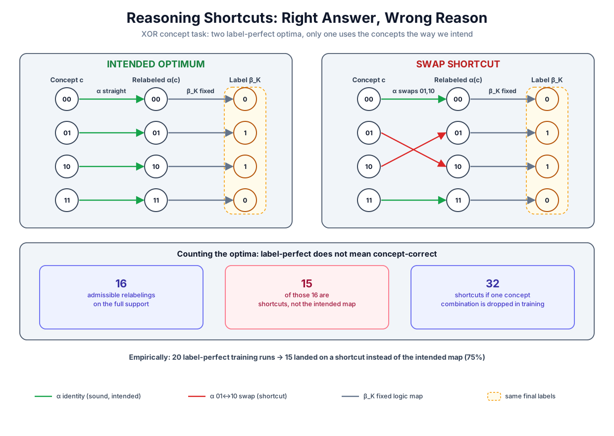 Two perfect optima of the same label likelihood: the intended identity map and the concept swap produce identical labels on every input, so no label metric can separate them.
Original diagram by the authors, created with AI assistance.
Two perfect optima of the same label likelihood: the intended identity map and the concept swap produce identical labels on every input, so no label metric can separate them.
Original diagram by the authors, created with AI assistance.
Counting the ways to be wrong
The commuting condition turns an amorphous worry into a finite combinatorial object, and the central result of the theory makes the risk exactly countable. Stated precisely, in our notation:
Theorem (shortcut count, stated without proof). For a deterministic knowledge over a finite concept space, and inputs that determine their ground-truth state (distinct states never generate the same input: the analysis's invertibility assumption A1, which the toy satisfies because its four corner clusters do not overlap), the deterministic optima of the label likelihood correspond to the relabelings that commute with on the observed support, and their number is
where is the set of all functions from to , the big wedge is logical "and" over every observed state, and is function composition ("apply , then "). Every admissible other than the identity is a reasoning shortcut, so the shortcut count is .
This theorem is imported, not proved here: it is Theorem 2 of the reasoning-shortcuts analysis, whose proof (that the deterministic optima are exactly these relabelings, no more and no fewer) is beyond this volume [1]. The sufficiency direction is the point-mass substitution derived in the previous section; the companion does not prove the theorem either, it evaluates it: the concept space has four states, so contains functions (four independent choices of image, one per domain state), few enough to enumerate outright (shortcuts.py, lines 116–132):
def admissible_alphas(support: list[tuple[int, int]]) -> list[tuple[int, ...]]:
    """Enumerate ALL deterministic relabelings α: 𝒢 → 𝒞 (tuples of image
    indices into COMBOS, one per ground-truth state, |𝒜| = 4⁴ = 256) and
    keep those label-indistinguishable from the truth on the observed
    support — the indicator inside Theorem 2's sum,
    N_opt = Σ_{α ∈ 𝒜} 1{ ⋀_{g ∈ supp(G)} (β_K ∘ α)(g) = β_K(g) }.
    Every admissible α except the identity is a reasoning shortcut; the
    support only constrains OBSERVED g's, so a smaller support means fewer
    conjuncts and strictly more surviving α."""
    supp = set(support)
    keep: list[tuple[int, ...]] = []
    for images in itertools.product(range(len(COMBOS)), repeat=len(COMBOS)):
        # (β_K ∘ α)(g) = β_K(g) for every OBSERVED g; unobserved g's are free.
        if all(beta_k(COMBOS[images[i]]) == beta_k(g)
               for i, g in enumerate(COMBOS) if g in supp):
            keep.append(images)
    return keep
For XOR the count also has a closed form we can derive completely. The label map partitions the four states into two fibers (preimage sets, the states sharing one label): the label-0 fiber and the label-1 fiber , each of size . The commuting condition constrains each observed state independently: may be any state in 's own fiber, which gives exactly choices. An unobserved state appears in no conjunct of the big wedge, so its image is unconstrained: choices. The choices multiply because a function is exactly one independent image per domain point. Write for the set of observed states and for its size, the number of observed states out of four; then
On the full support : . The committed run confirms the enumeration against the closed form:
[1] Theorem 2: count the alpha with (beta_K o alpha)(g) = beta_K(g) on all observed g
      support                |supp|  closed form     admissible  shortcuts
      full   00 01 10 11         4   2^4*4^0 =  16            16         15
      biased 00 01 -- 11         3   2^3*4^1 =  32            32         31
      dropping ONE observed combination doubles the optimum set (the EvenOdd move)
      example shortcuts admitted at full support:
        00->00 01->10 10->01 11->11   (the concept swap)
        00->11 01->10 10->01 11->00   (the double flip)
        00->00 01->01 10->10 11->00   (not even bitwise: 11 collapses onto 00)
      admitted ONLY under bias: 00->00 01->01 10->00 11->00
Sixteen perfect optima; one of them is the truth; fifteen are shortcuts. Walk one nontrivial survivor by hand, the concept swap , which exchanges the two mixed states and fixes the pure ones. Check the commuting condition at each of the four states:
| commutes? | ||||
|---|---|---|---|---|
| yes | ||||
| yes | ||||
| yes | ||||
| yes |
The swap survives because XOR is symmetric in its two arguments: swapping and can never change . A model that has learned "concept 1" to mean the true concept 2 and vice versa produces the correct label on every input that can ever exist, so the training loss, at its exact global minimum, holds the door open for it. Note what the concept swap is not: it is not the benign label-switching permutation Volume 4 measured and forgave. There, three anonymous topic clusters had no designated names, and any consistent naming was correct by construction. Here the two concepts have fixed, distinct intended meanings tied to input coordinates ( reads coordinate ), and the analysis is explicit on this point: a permuted-but-consistent concept map with a fixed intended semantics is still a shortcut [1]. The companion accordingly scores concepts against the ground truth as-is, with no re-alignment step (shortcuts.py, lines 280–307).
Support bias is a shortcut factory
The closed form has a lever in it, and it points the wrong way. Each observed state contributes a factor (constrained to its fiber); each unobserved state contributes a factor (unconstrained). Remove one state from the training support and its factor changes from to : the number of perfect optima doubles, from to . Fewer observations mean fewer conjuncts in the big wedge, and every conjunct that disappears frees a choice. Missing data does not merely weaken the statistics; it multiplies the population of models that are exactly right about everything they were shown.
The companion performs this move by dropping the single state from the support (shortcuts.py, line 352) and asserts the direction of the effect as a strict set inclusion, not just a bigger number (shortcuts.py, lines 362–368):
    full = admissible_alphas(COMBOS)
    biased = admissible_alphas(BIASED_SUPPORT)
    assert len(full) == 2 ** len(COMBOS) == 16
    assert len(biased) == 2 ** len(BIASED_SUPPORT) * 4 == 32
    assert IDENTITY in full, "the intended map must always be admissible"
    # The EvenOdd move: a smaller support strictly ENLARGES the optimum set.
    assert set(full) < set(biased) and len(biased) > len(full)
Every optimum of the full-support task remains an optimum of the biased task (removing constraints can never disqualify a survivor), and sixteen new ones join. The committed output prints one of the newcomers: the map sending , , , . Read it against the fibers: it fixes and , collapses onto (legal even on the full support, both carry label ), and sends , whose true label is , to , whose label is . On the full support that last move is fatal, one conjunct of the wedge fails. On the biased support the state is never observed, no conjunct mentions it, and a model that would mislabel if it ever appeared is a flawless optimum of the data it was given.
This is not a toy-only artifact; it is the move behind the field-scale demonstration. The reasoning-shortcuts study built MNIST-EvenOdd, a biased variant of MNIST addition (MNIST is the standard benchmark of handwritten digit images; the task labels a pair of digit images with their sum) in which only a fraction of the hundred digit combinations ever appears in training, and on it, state-of-the-art neuro-symbolic systems keep label F1 high while concept F1 collapses to nearly zero: the digit classifier inside the label-accurate adder has learned digits that are simply not the digits [1]. The table above is that experiment's combinatorial mechanism, small enough to enumerate.
| support | observed states | closed form | admissible | shortcuts |
|---|---|---|---|---|
| full | ||||
| biased |
Twenty seeds, fifteen shortcuts
Counting optima says how many ways training can go wrong; it does not say how often gradient descent does. A reasoning shortcut is a global optimum, so a single successful run demonstrates nothing about the risk, and a single failed run demonstrates nothing about its frequency. The honest protocol is a sweep: many training runs from independent random initializations, everything else held fixed [1]. The companion trains twenty seeds on the full-support XOR task, label supervision only, and scores each on held-out data: label accuracy and macro-F1 on (F1 is the harmonic mean of a class's precision and recall; the macro average is the unweighted mean of the per-class F1 scores, computed in macro_f1, shortcuts.py, lines 265–277), concept accuracy and macro-F1 on against the never-shown ground truth, and the empirical relabeling , read off as the modal (most frequently) predicted state of each true state's test cluster (shortcuts.py, lines 331–347 for the loop, 280–307 for the scoring). The committed sweep:
[3] the sweep: 20 seeds from label supervision only (concepts never shown)
      seed  F1(Y)  acc(Y)  F1(C)  acc(C)  learned alpha                verdict
         1  1.000  1.000   0.500  0.500   00->00 01->10 10->01 11->11  SHORTCUT
         2  1.000  1.000   1.000  1.000   00->00 01->01 10->10 11->11  intended
         3  1.000  1.000   0.000  0.000   00->11 01->10 10->01 11->00  SHORTCUT
         4  1.000  1.000   0.000  0.000   00->11 01->10 10->01 11->00  SHORTCUT
         5  1.000  1.000   1.000  1.000   00->00 01->01 10->10 11->11  intended
         6  1.000  1.000   1.000  1.000   00->00 01->01 10->10 11->11  intended
         7  1.000  1.000   0.500  0.500   00->00 01->10 10->01 11->11  SHORTCUT
         8  1.000  1.000   1.000  1.000   00->00 01->01 10->10 11->11  intended
         9  1.000  1.000   1.000  1.000   00->00 01->01 10->10 11->11  intended
        10  1.000  1.000   0.500  0.500   00->11 01->01 10->10 11->00  SHORTCUT
        11  1.000  1.000   0.500  0.500   00->00 01->10 10->01 11->11  SHORTCUT
        12  1.000  1.000   0.000  0.000   00->11 01->10 10->01 11->00  SHORTCUT
        13  1.000  1.000   0.500  0.500   00->11 01->01 10->10 11->00  SHORTCUT
        14  1.000  1.000   0.500  0.500   00->11 01->01 10->10 11->00  SHORTCUT
        15  1.000  1.000   0.733  0.750   00->00 01->01 10->01 11->11  SHORTCUT
        16  1.000  1.000   0.500  0.500   00->00 01->10 10->01 11->11  SHORTCUT
        17  1.000  1.000   0.200  0.250   00->11 01->10 10->10 11->00  SHORTCUT
        18  1.000  1.000   0.000  0.000   00->11 01->10 10->01 11->00  SHORTCUT
        19  1.000  1.000   0.733  0.750   00->00 01->01 10->01 11->11  SHORTCUT
        20  1.000  1.000   0.000  0.000   00->11 01->10 10->01 11->00  SHORTCUT
      RS frequency among near-optimal models (F1(C) under 0.95): 15/20 = 75%
      every learned alpha above is one of the 16 admissible maps Theorem 2 counted
Read the two metric columns against each other. The label column is a wall of : all twenty models are perfect on every held-out label, indistinguishable to any evaluation built on . The concept column is carnage: fifteen of twenty runs, 75%, land on a shortcut (the count the output's final line reports as the RS frequency, RS abbreviating reasoning shortcut), with F1(C) at , , , and five seeds at exactly . The learned maps decode the numbers. Seeds 3, 4, 12, 18, 20 found the double flip, bitwise negation of both concepts: every predicted bit is always wrong, so concept accuracy is exactly , while (the bar denotes bit negation; negating both inputs of XOR cancels) keeps every label right. Seeds 1, 7, 11, 16 found the concept swap walked above: each concept head is right exactly when , which is half the test set, so accuracy is . Seeds 15 and 19 found a map that is not even bitwise, collapsing onto : three states out of four survive intact, accuracy . And every one of the twenty learned maps, checked with cluster purity at least (purity is the minimum, over the four true states, of the share of that state's test cluster claimed by its modal predicted state; shortcuts.py, lines 299–305), is a member of the sixteen-element set the enumeration produced before training began (lines 394–397). The theorem's census predicted the sweep's entire menagerie.
The harness then pulls out one flagged seed and re-certifies its trained predictor against the circuit (shortcuts.py, lines 399–404), then prints the shortcut at full resolution (lines 461–468):
[4] caught in the act: seed 1 — F1(Y) = 1.000 with F1(C) = 0.500
      confusion, true concept state (rows) vs predicted (columns), test set:
               pred 00  pred 01  pred 10  pred 11
      g = 00       100        0        0        0
      g = 01         0        0      100        0
      g = 10         0      100        0        0
      g = 11         0        0        0      100
      the learned map is 00->00 01->10 10->01 11->11:
      the heads SWAPPED the two concepts — XOR is symmetric, so every label stays right
The matrix is as clean as a confusion matrix can be while being wrong: no scatter, no noise, four blocks of one hundred. Rows and sit on the diagonal; rows and have traded places wholesale. This model has not "roughly confused" the concepts; it has learned the swap exactly, with total confidence, as a global optimum of a loss it minimized perfectly.
The deployment reading is the reason this chapter exists. If the model is only ever used as a label machine, the shortcut is harmless by definition: the labels are right. But nobody builds a neuro-symbolic system to use it as a label machine. The concepts are the product: they are what gets transferred to a new task built on the same vocabulary (where suddenly fires on the wrong inputs), what an intervention edits ("set to 1 and re-run"), what an explanation exposes to a human ("the model concluded because and ", which is precisely backwards here). Every one of those downstream uses inherits the scramble, certified by a spotless label metric. Part I's faithfulness lesson recurs one level down: there, an explanation could misreport a model's mechanism; here, the model's own symbols misreport the world, and the metrics we ship with cannot see it.
Four factors govern the risk
The analysis identifies four factors that determine how many shortcuts a task admits and how likely training is to land on one [1]. Each has a named knob in the companion.
The knowledge . Shortcuts live in the fibers of the label map, so their number is controlled by how non-injective is. At one extreme, if were injective (every concept state its own label), each fiber would be a singleton, every observed state's factor would be , and on full support the count would be : the identity alone, no shortcuts possible. XOR is the fully balanced case for two bits: both fibers have size , and XOR's symmetry under swapping and under double negation is precisely what the sweep's favorite shortcuts exploited. Balance is not even the extreme for the count: AND, whose fibers are (size ) and (size ), admits deterministic optima on the full support by the same product of per-state fiber sizes; non-injectivity anywhere breeds shortcuts. Richer knowledge that distinguishes more concept states (adding a second label that breaks the symmetry, say ) shrinks fibers and kills shortcuts. The knob in the toy is beta_k itself (shortcuts.py, lines 77–80): the entire combinatorics of this chapter flows through that one small function.
The data support. Derived and measured above: each unobserved state's constraint factor relaxes from fiber size to full concept-space size, and the optimum set can only grow, here from 16 to 32 (shortcuts.py, line 352 and lines 362–368). Support bias is the factor a practitioner controls least and audits least; the biased MNIST split shows it acting at field scale [1].
The objective. Everything above assumed the loss is label likelihood alone, the sup_idx=None path of the companion's loss (shortcuts.py, lines 193–221). Any objective term that touches the concepts directly changes the optimum set itself: the mitigation below is exactly such a term, and the next chapters measure a second one (an entropy term that prefers deterministic, disentangled concepts among the optima).
The architecture. The relabelings counted by the theorem are those the extractor can realize, and this is where architecture enters the count: through the candidate set the sum ranges over. The theorem above took to be all functions because the companion's extractor can realize every one of them. That extractor has factorized output heads: two independent softmax heads, one per concept, but both reading the same shared features of the whole input (shortcuts.py, lines 150–155). This is not what the analysis calls disentangled. Its definition requires the concept distribution to factorize as , where is the learned concept vector and the ground-truth state (both viewed as random variables), the subscript picks out the -th concept and its matching ground-truth factor, and multiplies over the concepts: each learned concept must be computed from its own part of the input [1]. The companion's heads violate that (in the learned swap, head 1 computes the true concept 2, and both heads read both coordinates), which is how 15 of 20 seeds could find a shortcut. An extractor that restricts each head to its own input coordinate is disentangled in this sense, and the analysis's first experimental finding is how much that buys: on XOR-style tasks with exhaustive support, disentanglement alone drops the shortcut frequency from 100% to 0% for every backend tested, because collapses from all functions to products of per-concept maps and the swap stops being representable. Beyond fixing , architecture also shapes how the optimizer's basin sizes distribute over the maps that remain; the identifiability chapters make this factor measurable.
The first repair: a few concept labels
If label likelihood cannot distinguish the sixteen optima, add a term that can. The most direct lever, and the one the analysis found necessary for its DeepProbLog-style backend (its mitigation study's overall verdict is that no strategy alone suffices for every method it tests) [1], is concept supervision: ground-truth concept labels on a small fraction of the training points. The companion labels 12 of its 120 training points (10%, stratified: three per concept state; shortcuts.py, lines 315–321) and adds, per head , a cross-entropy on the supervised subset (the set of supervised training indices). In the excerpt, is head 's softmax output vector over its concept's two values, and is training point 's true bit for concept :
    if sup_idx is not None:
        m = len(sup_idx)
        for j, (pi, u) in enumerate(((pi1, u1), (pi2, u2))):
            hit = np.maximum(pi[sup_idx, g[sup_idx, j]], EPS)
            # L_c per head = −(1/m) Σ_{i∈𝒮} log π_j[g_{ij}], weighted by w_c.
            total += W_C * float(-np.log(hit).mean())
            # ∂(w_c·L_c)/∂π_j[g_{ij}] = −w_c/(m·π_j[g_{ij}]) on supervised rows.
            u[sup_idx, g[sup_idx, j]] += -W_C / (m * hit)
(shortcuts.py, lines 223–230; the added gradient route is certified by the same finite-difference check as the base loss.) Why this works is transparent in the relabeling picture. Take a shortcut and a supervised example whose true state is with . The extractor that realizes puts probability near on the true state's entry for at least one head, so the term is driven toward infinity: is no longer an optimum of the combined objective. Each supervised state therefore pins , cutting that state's choice factor from its fiber size to . In the closed form, supervising all four states (which the stratified 10% sample achieves) takes the surviving count from to : only the identity remains. A dozen cheap labels collapse the entire shortcut population, not by making the optimizer smarter but by changing which parameterizations count as perfect.
The committed measurement, on the very seed caught above, same initialization, same epochs, only the 12 concept labels added:
[5] mitigation (Prop. 5): concept labels on 12/120 training points, same init
      seed 1    F1(Y)   F1(C)   acc(C)   learned alpha
      before    1.000   0.500   0.500   00->00 01->10 10->01 11->11
      after     1.000   1.000   1.000   00->00 01->01 10->10 11->11
      10% concept supervision restores the intended semantics; labels stay perfect
Concept F1 goes from to ; the learned map returns to the identity; label F1 never moves off (shortcuts.py, lines 407–409 assert the identity map and near-perfect label and concept accuracy). This is the mitigation lever at its cheapest setting, one task, one seed, one fraction. How the required fraction scales, what the other levers (entropy regularization, multi-task knowledge, ensembles) buy, and what can be guaranteed rather than observed: that is the quantitative program of the identifiability chapter, where this before/after pair becomes a table.
The unsolved part
The counting theorem is exact, and that exactness rests on two assumptions the toy satisfies and the frontier does not. First, the concept space must be enumerable: the sum over ranged over candidate relabelings, but for twenty binary concepts, and , far beyond enumeration (the successor chapters count admissible relabelings with #SAT solvers, propositional model counters that count a formula's satisfying assignments rather than finding one, instead of loops, which extends the reach but not indefinitely). Second, and more fundamentally, the knowledge and the intended concept vocabulary must be known: the census of wrong meanings is computed against a fixed catalogue of right ones. A modern system whose concept vocabulary is itself learned, a foundation model's emergent features, say, offers no to commute with, so the theory can name the disease but not count its strains. The live problem is therefore detection without concept labels: deciding, from a trained model's behavior alone, whether it sits on a shortcut. The sweep needed ground-truth concepts to fill in its F1(C) column; in deployment that column is blank by definition. The current line attacks the problem through uncertainty: a model cannot know which of several admissible relabelings it should have learned, so an ensemble over the optima should be maximally uncertain about concepts exactly where shortcuts live, and calibrated concept ensembles built on this idea (BEARS, short for "BE Aware of Reasoning Shortcuts") turn shortcut risk into a measurable confidence signal [3]. That converts the problem of this chapter into the problem of the calibration chapter, which is one reason this volume treats them as one arc. And the honest close: nothing in this chapter's mechanism was specific to XOR, to two concepts, or to twenty seeds. Every Volume 4 success that trained latent concepts through logic, the DeepProbLog family first among them [4], owes its concept semantics to luck, architecture, and data support until an audit of this kind has been run. Our own 100% topic recovery survives only because its topics were anonymous: there a consistent permutation is correct by construction, and the Volume 4 module measured exactly that residual freedom. Any success whose concepts carry fixed intended meanings needs this chapter's as-is audit, which is precisely the audit the XOR miniature ran, and which fifteen of twenty label-perfect seeds failed.
Why it matters
This chapter is the hinge of the volume's trust story. Part I asked whether we can trust explanations of a model's reasoning; the reasoning shortcut shows the question goes deeper, because the model's internal symbols themselves can be systematically wrong while every output is right. For the series' arc, it re-prices Volume 4's central promise: distant supervision does convert task labels into symbol-level training signal, but the conversion is underdetermined, and the knowledge that made the labels cheap is the same knowledge whose symmetries make the symbols ambiguous. For the reader's own research, the operational lessons are blunt. Report sweeps, not runs, when latent concepts are involved; a single seed's concept accuracy is an anecdote about one basin. Audit the support: the count doubled the moment one combination went missing, and real datasets are missing combinations everywhere. Treat label metrics as exactly what they are, functions of that are constant across all admissible optima, and budget for the cheapest thing that is not one: a handful of concept labels bought back the entire semantics here for 10% of the data. And when concepts will be transferred, intervened on, or shown to a human, demand the confusion matrix against ground truth somewhere, on some subset, before believing it anywhere.
Key terms
- Reasoning shortcut (RS): a parameterization that maximizes label likelihood while its concept distribution differs from the ground truth; an unintended optimum, right on every label for wrong reasons.
- Label map : for deterministic knowledge, the function sending each concept state to the label the knowledge assigns it; here .
- Relabeling : a function from ground-truth concept states to model concept states describing a systematic semantic error; admissible (an optimum) when it commutes with on the observed support.
- Fiber: the set of concept states sharing one label, ; observed states may be relabeled only within their fiber, so fiber sizes drive the shortcut count.
- Support (of the concept distribution): the set of concept states that actually occur in training; unobserved states impose no constraint on , so a smaller support strictly enlarges the optimum set.
- Counting theorem: the imported result that deterministic optima correspond exactly to admissible relabelings, making the shortcut count computable by enumeration (here) or #SAT (at scale).
- Concept supervision: direct concept labels on a subset of training points; each supervised state pins at that state, cutting its choice factor to 1 and, with all states covered, leaving only the identity.
- Disentangled extractor: an extractor whose concept distribution factorizes as , each concept computed from its own part of the input; the companion's shared-feature heads are not disentangled, and architecture enters the count by fixing the candidate set of realizable relabelings.
Where this leads
This chapter established that the optima of label likelihood form a set, counted it, and watched training sample from it. The natural next question is the converse: under what conditions does the set shrink to one, so that maximizing the likelihood provably recovers the intended concepts? That is an identifiability question, the same shape as asking when a statistical model's parameters are determined by its distribution, and it has quantitative answers: how much concept supervision, how many tasks sharing a vocabulary, which properties of buy uniqueness, and what the mitigation table looks like when every lever is measured on common ground. Identifiability takes up exactly that, beginning with the theorem this chapter kept promising: that no function of the labels alone, however clever, can detect the difference this chapter spent its pages making visible.
Companion code: examples/frontier/shortcuts.py implements the four-world predictor with its Volume 4 circuit certification, the relabeling enumeration behind the counting theorem, the full-versus-biased support comparison, the twenty-seed sweep, and the concept-supervision mitigation. Run python3 examples/frontier/shortcuts.py to reproduce every number in this chapter; the run is deterministic and every claim is guarded by an assert.