Open Problems: The G1–G8 Gaps

📍 Where we are: Part VIII · The Research Runway — Chapter 21. The Eight Claims closed Part VII by freezing a claims-to-experiments matrix and running its honest toy subset; this chapter turns the same discipline outward, from what one system claims to what the whole field cannot yet do.

Every research field carries a list of open problems, and most such lists are wishes: "systems should be more robust," "explanations should be more trustworthy." A wish cannot fail, so a wish cannot guide work. This chapter states the neuro-symbolic field's open problems the way the previous chapter stated a system's claims: as capability gaps, differences between what has been demonstrated and what is needed, each with a named instrument that would measure progress and a falsifiable notion of "closed." The eight gaps G1 through G8 come from the survey corpus behind the capstone, the same gap analysis that motivated SATORI's design, and this chapter gives each one the identical four-part treatment: the precise statement, the best partial answers with their committed or cited evidence, the measuring instrument, and a difficulty estimate stated concretely enough to be argued with. The volume's twist is that the partial answers are not hypothetical: for every gap, some chapter of this series built or cited the current best evidence, so the gap map doubles as an index into everything the five volumes measured.

The simple version

Imagine a mountaineering club's ledger of unclimbed faces. A useless entry says "the north face is very hard." A useful entry says: the face is 900 meters; the highest camp anyone has reached is at 610 meters, established by the Larsen route in 2019; the next 120 meters are blank ice where every attempt has turned back; progress will be measured by fixed anchors above camp three; and the grade is disputed between 5.11 and 5.13, so bring evidence. The second entry names what has been done, what stops everyone, and exactly what would count as getting higher. This chapter writes the second kind of entry, eight times, for the eight faces the neuro-symbolic field has not climbed.

What this chapter covers

• The framing move: open problems as capability gaps with instruments rather than wishes, the discipline inherited from the claims chapter, and the eight-gap map with its provenance in the field surveys and in the capstone's own source corpus.
• G1 and G7, the trust pair: the exact/learnable split stated sharply with the Volume 4 ledger recalled, calibration-under-shortcuts as its measurement problem, and the identifiability bar that defines "closed."
• G2 and G4, the learning pair: the rule-search explosion quantified on this series' own template counts, routing and query-conditioned generation as partial answers with an unproven systematicity claim, and ontology-blind learning with its grounded-embedding partial fix.
• G3, the systems gap: the CPU/GPU asymmetry with Part IV's committed numbers and cited ceilings, and the wall named precisely: dynamic sparse frontiers versus SIMD batches, with the depth physics underneath.
• G5 and G6, transfer and explanation: what moves across ontologies today and what does not, the unfaithfulness evidence and the traces-by-construction partial answer, and the instruments both gaps already have.
• G8, the meta-cognition gap: the thin slice of the literature, what Part III's abstention machinery actually provides, and why this gap compounds all the others.
• The runway assembled: the eight gaps ranked on two axes, instrument-readiness and dependency, ending with the reader's own exit: pick a gap whose instrument exists and whose dependencies are met.

Problems stated as gaps, not wishes

The framing move is inherited from two places. The first is the previous chapter's claims discipline: a claim well stated names the experiment that would refute it, and the honest run of satori_eval.py sorted eight claims into toy-verified with a number and cited-only with a reason. An open problem deserves the same grammar in reverse. A problem well stated names the experiment that would close it: the capability that is missing, the strongest partial demonstration on record, and the measurement that would register the difference. The second inheritance is the field's own survey literature, which has been converging on this list for years: the third-wave analysis that named learning-versus-reasoning integration, extrapolation beyond the training distribution, and sound explanation as the standing challenges [1]; the taxonomy of integration patterns that showed how many architectural answers already coexist, each buying a different corner of the problem [2]; the design-space survey that mapped which combinations of logic, probability, and learning have actually been built, and where the map runs out [3]; and the boxology of hybrid design patterns, which gave the recurring system shapes names precise enough to be reused as engineering vocabulary [4].

The eight-gap map G1 through G8 is the SATORI corpus's distillation of that literature into rows sharp enough to build against, and it has been sitting inside this volume's companion suite all along. The capstone evaluator carries the map in its own docstring, together with an honest statement of which gaps its toy run exhibits and which it can only cite (examples/frontier/satori_eval.py, lines 46–52):

The gap map G1–G8 of ``../satori/docs/RELATED_WORK.md`` — G1 exact/learnable
split, G2 rule-search explosion, G3 CPU-bound symbolic inference, G4
ontology-blind rule learning, G5 non-transferability, G6 explanation
faithfulness, G7 uncertainty/calibration/shortcuts, G8 meta-cognition — is
the open-problems chapter's syllabus; this module exhibits G1 (C2), G2 (a
25-template space, no enumeration blow-up), G4 (C1's substrate is the TBox
kernel), G6 (C3) and G7/G8 (C5), and leaves G3/G5 to the citations above.

That comment is this chapter's table of contents. One run of the module (cd examples/frontier && python3 satori_eval.py) prints the claims table the previous chapter read, and its verified/cited split is exactly the gap map's evidence inventory at toy scale:

  C1 multi-hop EPFO answering   toy-verified  MRR 0.568 vs random 0.230 / oracle 1.000
  C2 router learns rules        toy-verified  advises∘advises recovered, α = 0.972, exact decode
  C3 faithful proof traces      toy-verified  comp 8/8, suff 4/4, trace ⊇ MinA 2/2
  C4 GPU-batched scalability    cited-only    proxy gpu_fixpoint.py; needs PyReason/Scallop at scale
  C5 calibration + abstention   toy-verified  ECE 0.019; coverage 0.821 @ acc-on-answered 1.000
  C6 ontology grounding Δ MRR   cited-only    ablation degenerate here; Box2EL / TransBox carry it
  C7 cross-ontology transfer    cited-only    needs a 2nd ontology; RRN is the failing baseline
  C8 crisp soundness (τ→0)      toy-verified  satori_lite re-run: Horn 47/47, EL 46/46, complete iff L ≥ 3

Every "toy-verified" row is a partial answer to some gap; every "cited-only" row marks where the gap's instrument does not yet fit in a laptop-sized world. The table's shorthand is the previous chapter's, decoded once here: MRR is the mean reciprocal rank, the ranking metric that averages one over the rank of each true answer; EPFO queries are existential positive first-order queries, the multi-hop query class C1 answers; and in the C2 row, the ∘ of advises∘advises is relation composition (apply advises, then advises again), α is the router's attention weight on that true rule body, and τ is the temperature whose zero limit makes C8's kernel crisp. The rest of this chapter walks the eight gaps in pairs and singles, in the order their dependencies suggest, and holds each to the four-part treatment promised above.

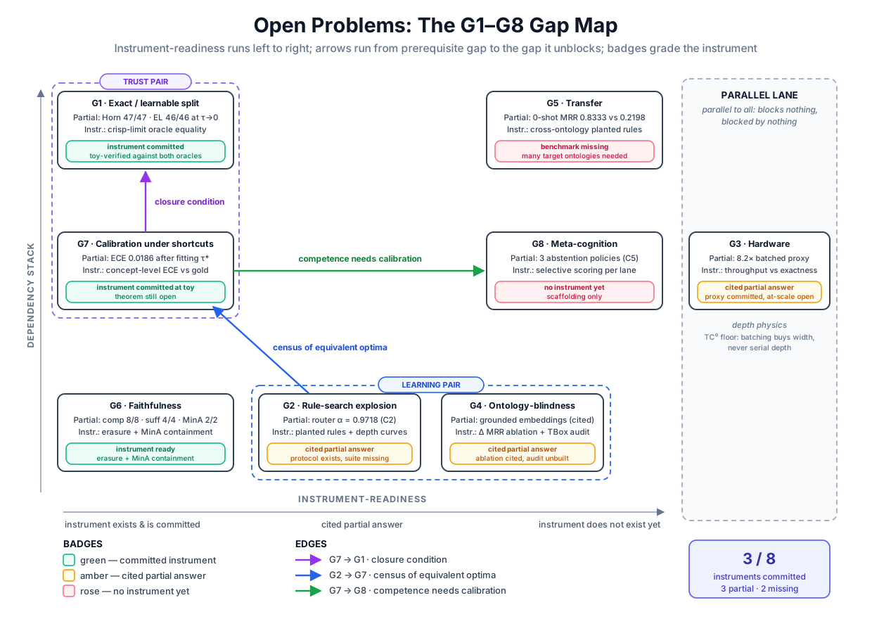The eight gaps as a dependency-ordered map: each card names its best partial answer and its instrument, arrows mark which gaps block which, and the color badges grade instrument-readiness. Original diagram by the authors, created with AI assistance.

G1 and G7: the trust pair

G1, the exact/learnable split, stated precisely. Existing systems occupy two corners and not the space between. In one corner sit the exact reasoners: ELK, HermiT, Konclude (Volume 2's EL reasoners and DL engines), the annotated-logic engines; sound and complete over their fragments, every answer a theorem, and fixed, with hand-authored rules and no gradient anywhere. In the other corner sit the trainable systems: fuzzy compilations, soft provers, query embeddings; every parameter learnable and no answer a theorem; the two corners and the empty middle between them are the design-space survey's own map [3]. The gap is a system that is simultaneously trainable and sound, and Volume 4's closing ledger measured what each corner pays. The trainable corner pays in meaning: the same two-step citation chain came out as 0.80, 0.72, or 0.70 depending on a t-norm choice the logic cannot adjudicate, three defensible confidences for one conclusion (the committed tnorms.py chain in Volume 4's verdict). The exact corner pays in scale: the gradient of exact inference can be had, certified against finite differences to 2.7e-13 in the committed DeepProbLog miniature, but the grounding-and-compilation bill that buys it grows with problem size until, in the successor evaluations that chapter cites, the exact pipeline times out near four-digit MNIST addition. Every framework in that volume paid one side of this split; none escaped it.

The partial answer with its committed evidence. Annotated differentiable substrates, the line this series built toward Part VII, hold both corner properties at their limits: the capstone kernel is differentiable everywhere (its router trained by plain gradient descent, hand gradients checked to 1.17e-11) and provably crisp at the temperature limit, recovering the Horn closure 47/47 and the EL closure 46/46 against both classical oracles, complete exactly when the unroll depth reaches the saturation depth (the C8 row above). That is a genuine occupancy of the middle: sound at τ→0, trainable at τ above 0. What it is not is a closure of the gap, because between the limits sits an open calibration debt: the kernel's soft degrees are only usable as confidences after a fitted temperature (the committed ECE (expected calibration error) of 0.0186 on 306 imputation-needing pairs required calibration.py's $\tau^* = 1.4172$ first), and nothing yet proves those calibrated degrees track the concepts rather than the labels. Which is exactly where the split's measurement problem lives, and that problem has its own row on the map.

G7, calibration under shortcuts, stated precisely. Part II proved that naive confidence cannot certify concepts: for a deterministic knowledge (the fixed symbolic program mapping concept states to labels) with non-singleton fibers (a fiber is the set of concept states that produce the same label), the label likelihood has multiple global optima that differ only in what the internal symbols mean, sixteen admissible relabelings on the XOR task's full support, fifteen of them wrong, with twenty label-perfect training runs landing on a shortcut fifteen times [5]. A confidence read off such a model is confidence in the label, and the committed contrast in the rsbench chapter shows what that costs: the shortcut model's concept-level expected calibration error is 0.2467 against its supervised twin's 0.0013, confident and wrong about meaning by a factor of about 190. G7 is the gap between confidence that tracks answers and confidence that tracks the concept-grounding underneath them. Its first partial answers exist: shortcut-aware calibration in the BEARS line ensembles concept posteriors so that shortcut ambiguity surfaces as concept-level uncertainty an abstention gate can read, the proposal Part III's abstention chapter cited as the symptomatic treatment; and the identifiability chapter priced the causal treatments, factorized heads cutting XOR's sixteen admissible maps to two and twelve stratified concept labels leaving the identity alone.

What closed would look like. The bar is the identifiability bar restated as a calibration property: a trainable system whose reported uncertainty provably covers the surviving symmetry orbit, so that when the knowledge's symmetry group is trivial on the observed support the confidence converges to concept-grounded probability, and when it is not, the reported concept uncertainty is at least the orbit's ambiguity. The conjecture that calibration tracks identifiability is stated in the identifiability chapter and proved nowhere. The instrument exists at benchmark scale (concept-level ECE against gold concepts, rsbench's panel); the theorem does not. Difficulty estimate, stated to be argued with: the instrument work is a one-to-two-year project for a single group, because the metrics and testbeds are built; the theorem connecting calibration to the symmetry group is harder, since it must quantify over training dynamics, not just optima, and nothing in the current theory addresses which optimum gradient descent selects. A reviewer who thinks the theorem is five years away rather than two should point at the missing selection theory; a reviewer who thinks it is one should name a proof strategy for non-enumerable concept spaces.

G2 and G4: the learning pair

G2, rule-search explosion, quantified on this series' own numbers. A rule learner that enumerates candidate bodies pays exponentially in rule length. The counting is elementary and worth doing on the running example. With 5 base roles, the length-2 chain bodies number $5^2 = 25$; that is the template space the capstone's router searched, and the companion holds it as a literal product (examples/frontier/satori_eval.py, lines 154–159):

# --- C2: planted-rule recovery by a softmax router --------------------------------
# The template space: every length-2 role chain  r(x,y) ∧ s(y,z) → head(x,z)
# over the 5 base roles — 25 candidate rule bodies, one of which (advises ∘
# advises) is the grandAdvisor rule the router is never shown.
TEMPLATES: list[tuple[str, str]] = sorted(
    itertools.product(kg.RELATIONS, kg.RELATIONS))

Volume 4's Neural-LP chapter worked with the richer operator vocabulary the real systems use, 11 operators (5 relations, 5 inverses, the identity), so its length-$T$ body space is $11^T$: 121 bodies at two hops, 1,331 at three, 14,641 at four, and the attention trick is precisely a way to score this space without listing it, holding $T$ softmax distributions instead of $11^T$ confidences. The exponential does not disappear; it moves into the size of the hypothesis space the soft weights must implicitly rank, and it is joined by a second, sharper wall: the chain bias. Everything expressible as a product of adjacency matrices is a single path of fresh variables; rules whose bodies branch, compare siblings, or close a cycle are outside the searched space at any length. The gap is a rule learner whose search scales past both walls.

The partial answers and their unproven half. Routing is the first: the committed C2 row shows a softmax router over the 25 templates recovering the hidden grandAdvisor rule exactly, attention 0.9718 on the true body, from three query answers and hand-derived gradients. Query-conditioned composition is the second: the CTP (Conditional Theorem Prover) and R5 line of query-conditioned provers, met in Volume 4's neural theorem proving chapter, selects rule subsets per reasoning step instead of enumerating bodies [6], a line this series' source corpus reads as the field's live attempt at systematic generalization. The unproven half is the word systematicity itself. Recovering a planted rule inside a handed-to-you template space, which is what both our C2 and the published planted-rule results demonstrate, is not compositional generalization; the claim that routed rule pieces recombine correctly on deeper, unseen compositions is exactly the claim a CLUTRR-style probe tests (Compositional Language Understanding and Text-based Relational Reasoning: train on short kinship compositions, test on strictly longer ones), and it is on such depth-generalization curves, not on planted-rule recovery, that the routing line's systematicity must be judged; it has not been. The instrument, then, already has a form: planted rules plus held-out composition depths, scored as exact-recovery and depth-generalization curves. Difficulty estimate: demonstrating some systematic router on synthetic worlds is near-term (the pieces exist in this series' own companions); doing it with a hypothesis space that includes branching and cyclic bodies, where no matrix-product shortcut exists, has no published path at all, and a reviewer should treat any proposal that keeps the chain bias while claiming general rule learning as overclaiming by construction.

G4, ontology-blindness, stated precisely. The rule learners above consume a bag of edges. Handed the academic world's knowledge graph, Neural-LP sees 15 triples; it does not see that advises is asserted between a Professor and a Student, that TenuredStudentAdvisor is unsatisfiable, or any other consequence of the 14-axiom TBox that Volume 2's oracle derives. The TBox is a strong prior over which rules can be true, and the learners that dominate knowledge-graph completion ignore it entirely; that observation is the gap map's own G4 row. The partial answer arrived from the geometric side: Volume 3's Part III built the EL embeddings, Box2EL, and TransBox line, in which TBox axioms become geometric containment constraints and the published ablations show ontology grounding paying measurable ranking improvements where it has been tested. But grounding an embedding before learning is the easy half. The open joint problem is learning rules while reasoning over an expressive fragment, EL and up, so that a candidate rule inconsistent with the TBox is never entertained and a derived subsumption can serve as training signal mid-run. The capstone is honest about how far the toy evidence reaches: its C6 row is cited-only, because a kernel built from the TBox cannot run the on/off ablation that would isolate grounding's contribution; the ablation needs embeddings that could ignore the ontology, and it lives at Box2EL/TransBox scale. Instrument: the Δ MRR ablation (grounding on versus off, same architecture) plus a consistency audit of learned rules against the TBox. The first exists in the cited papers; the second is cheap to build and, to this series' knowledge, unreported. Difficulty: the audit is a student project; joint learning-and-reasoning over EL with soundness intact is a multi-year program, because it needs G1's substrate as a prerequisite.

G3: the systems gap

Stated precisely. Learning rides accelerators; symbolic inference, in the mainstream engines, does not. The design-space survey states the soft half of that sentence: exact probabilistic inference is computationally expensive, and scaling it is a standing open challenge [3]. The sharp half is the engines' own record, collected in the gap map's source corpus: the annotated-logic and probabilistic-logic families, PyReason, DeepProbLog, and Scallop among them, keep their symbolic cores CPU-bound with no batched inference, while every neural baseline in this series trained on hardware built for dense regular arithmetic. The gap is exact inference that saturates the same silicon.

The live front, with Part IV's numbers. The GPU reasoning chapter showed the shape of the answer at toy scale: Volume 2's EL completion re-expressed as boolean matrix algebra, asserted cell-for-cell equal to the classical oracle on the real TBox and three seeded synthetic ones, semi-naive deltas cutting derivation events from 71 to 28, and one hundred stacked ontology variants closed in a single loop-free tensor pass, about 8.2 times faster than the Python loop on the committed CPU-NumPy proxy. The cited ceilings mark where that shape has been industrialized: the parallel-materialization line behind RDFox measured speedups up to 87-fold on a 128-core machine, and KLay layerizes irregular arithmetic circuits into dense per-level tensor operations for accelerators, the same move one level down (both cited in Part IV). So the front is live in both directions, logic-to-tensors and circuits-to-tensors.

The wall, named precisely. It is a data-structure problem underneath a hardware problem. A saturation frontier is dynamic and sparse: the committed wavefront on the academic TBox is 9, 12, 7, 0 new consequences per wave, a set that grows, crests, and empties. SIMD (single instruction, multiple data) hardware wants the opposite, wide regular batches known in advance; the toy papering-over (recompute densely every wave) is only sane because the matrices are tiny. Nobody has a settled design for a derivation frontier that stays resident and efficient on an accelerator as it sparsifies, and deletion (the DRed machinery of the materialization chapter) has no accepted batched formulation at all. And beneath the engineering sits physics that no amount of it can repeal. The parallelism tradeoff proved that log-precision transformers lie inside uniform TC⁰, the class of constant-depth, polynomial-size threshold-circuit families [7], and the same containment argument extends to any similarly constant-depth batched substrate; stated precisely, any function such a model computes on inputs of length $n$ is computable by a circuit family whose depth is a constant independent of $n$, whose gate count grows at most polynomially in $n$, whose gates include thresholds (a threshold gate fires exactly when at least $\theta$ of its input wires carry 1), and whose members are all produced by one simple uniform recipe. The proof is beyond this volume; the depth-ceiling chapter states it with every symbol decoded, and its companion demonstrates the mechanism instead, trained cliffs that move with depth but never disappear. The consequence for G3: since PTIME-complete closures (saturation problems as hard as any problem solvable in polynomial time; the depth-ceiling chapter decodes both P and completeness) are outside TC⁰ unless conjectured hierarchies collapse, batching buys back constants and parallel width, never the serial depth of the non-linear core. Difficulty: the sparse-frontier kernel is a systems thesis, hard but bounded; the depth axis is not an engineering problem at all, and proposals should say which side of that line they live on.

G5: the transfer gap

Stated precisely. Reasoning machinery trained on one ontology should move to another; today, almost none of it does. The classical negative exhibit is the RRN (Recursive Reasoning Networks) line, deep emulators of the OWL 2 RL rule profile (OWL is the Web Ontology Language) retrained per domain, which is why the capstone's C7 row is cited-only with RRN named as the failing baseline. What transfers today is structural link prediction: Volume 4's foundation-model chapter committed the receipt at toy scale, a twelve-parameter projector trained only on the academic world scoring zero-shot MRR 0.8333 on a disjoint-vocabulary hospital world against a 0.2198 random floor, and the cited benchmark-scale result is stronger, zero-shot 0.395 average MRR beating per-graph-trained baselines at 0.344. What does not transfer is everything this volume added on top: proof structure, rule repertoires, calibration temperatures. A vocabulary-independent substrate moves the scorer; nobody has shown it moves the derivations.

The instrument and the honest difficulty note. The instrument is this volume's own planted-rule protocol lifted to two vocabularies: plant a rule in ontology A, train the router there, and score exact rule recovery and proof-trace quality on ontology B, whose relation names share nothing with A, using the C2 decode-and-compare machinery and the C3 erasure-plus-MinA kit unchanged. The two-world pair for it already exists in the companion suite (the academic and hospital graphs of ultra_lite.py). What does not exist is the benchmark that would make a transfer claim mean something: transfer needs many target ontologies spanning size, depth, and fragment, the way GALEN, Gene Ontology, and SNOMED CT span the EL world, and no such cross-ontology reasoning-transfer suite has been assembled. The scarcity is acknowledged inside the SATORI plan itself, which lists curating ontology-enriched query sets as a contribution precisely because it does not exist to borrow. Difficulty: the two-vocabulary demonstration is near-term; the benchmark is a community-scale effort, and a reviewer should discount any transfer claim evaluated on a single target as one anecdote.

G6: the explanation gap

Stated precisely. Systems that explain themselves for free, by exposing attention maps or generated chains of thought, are documented to explain unfaithfully: the artifact shown is not the reason for the answer. Part I built the committed construction: a classifier whose attention piles 0.5673 of its mass on a feature whose erasure moves the output by 0.0004, while the actually-used feature carries a trained weight of 7.7077 and one twelfth the attention; the faithfulness chapter measured the mismatch with ERASER-style comprehensiveness (attention rationales 0.2497 against occlusion's 0.3659 and a 0.0789 random floor) and cited the at-scale evidence for both attention maps and chains of thought. The gap is explanation that is guaranteed to be the reason, at the scale where explanations matter.

The partial answer, and the ablation nobody has run. Traces-by-construction is the live line: architectures where the explanation is the computation, so faithfulness is structural rather than measured. The capstone's C3 row is the committed miniature, scored against the MinA (minimal axiom set, the justifications chapter's ground-truth explanation unit) and quoted from the run:

[3] C3 — faithful traces: erasure + MinA containment
  Horn face, 4 derived atoms — e.g. grandAdvisor(alice, carol) has trace leaves advises(alice, bob), advises(bob, carol)
    comprehensiveness 8/8: every leaf deletion kills its atom; leaves ALONE re-derive it (4/4)
    12 seeded non-trace deletions (default_rng(5)): nothing breaks (asserted)
  TBox face — the discretized trace vs justifications.py:
    Professor ⊑ Researcher: trace axioms {1} ⊇ MinA {1}   (all MinAs: {1} {4, 5})
    TenuredStudentAdvisor ⊑ ⊥: trace axioms {6, 10, 11, 12} ⊇ MinA {6, 10, 11, 12}   (all MinAs: {6, 10, 11, 12})

Read the trace as the gap's best current evidence: every trace leaf is causally necessary (deleting any of the 8 breaks its atom), the leaves alone are sufficient, non-trace deletions change nothing, and the discretized ontology trace contains a true minimal justification found independently by the hitting-set tree of the justifications chapter; the block's trace ⊇ MinA lines record exactly that containment, the trace's axiom set holding a complete MinA as a subset. That is faithfulness by construction, verified by instrument, at 13 entities. The open question is whether trace quality survives training pressure at scale: when the same architecture is trained hard on answer accuracy, does the trace stay minimal and causal, or does optimization learn to route real computation around the legible path while the trace decays into decoration? That interaction ablation, trace-faithfulness metrics measured across a training run on a benchmark-scale system, has not been published by anyone, and it is the single experiment this gap most needs. The instrument requires no invention: erasure plus MinA containment is this volume's own kit, and it runs on anything that emits a discrete trace. Difficulty: the ablation is a one-year project for a group with a trace-emitting system; making traces-by-construction cheap at scale is G3's problem wearing G6's clothes, which is why the runway section draws an edge between them.

G8: the meta-cognition gap

Stated precisely. Knowing-when-you-don't-know occupies a sliver of the neuro-symbolic literature; the survey corpus behind the gap map counts meta-cognition at roughly five percent of the work it reviews [8], the map's thinnest slice, and the field-level analyses that seeded the map file trust and self-knowledge among the standing challenges, never the achievements [1]. The temptation is to read Part III as having closed it, and the precise statement of the gap is exactly why it did not. What exists is abstention machinery: policies that decline questions based on scores, intervals, or structure. Part III's committed three-policy table put them on one axis, the Chow threshold at coverage 0.9841 with a silent-wrong rate of 0.0159, the open-world interval at coverage 0.8651 with zero silent errors, the structural parser at 0.9293 with zero by construction; and the capstone's C5 row re-ran the interval species end to end:

[4] C5 — calibration + open-world abstention
  kernel degrees on the 306 imputation-needing (query, entity) pairs: ECE = 0.0186
  interval [ℓ, u]: ℓ from G_train, u from the 62-edge typed completion (⊇ all 18 true edges)
  policy                    coverage   acc-on-answered
  closed-world traversal      1.0000   0.9487   (24 errors = 23 hard answers + the 2in witness)
  interval + abstain          0.8205   1.0000   (19 yes + 365 no; abstains 84/468)

Read the block's notation off the claims chapter's setup: each answer's truth is bracketed by an interval whose lower bound ℓ comes from G_train, the 15-edge training graph of observed edges, and whose upper bound u comes from the 62-edge typed completion, every edge the TBox's types allow; the ⊇ records that this completion contains all 18 true edges as a subset; and 2in names the one query shape, an intersection of two branches with one branch negated, on which the closed world manufactures its wrong yes.

What the gap actually asks is a level up from any of that. An abstention policy consumes a per-question signal and declines a question. A meta-cognitive system models its own competence boundary, the region of inputs where its machinery is reliable, and routes accordingly: this query lies inside my sound fragment, answer symbolically with a proof; this one needs imputation, answer neurally with a calibrated degree; this one is outside both, decline or escalate. The concrete next artifact is exactly that neural-versus-symbolic router, and it is not exotic: the boxology's meta-reasoning-for-control pattern already puts a symbolic controller above a learner, reasoning about the learner's state and steering its behavior [4], and the per-input routing G8 needs is a short, still-unnamed step beyond that pattern; what is missing is the trained boundary model and the evidence standard for it (a routing system should be scored like a selective predictor, coverage per lane, risk per lane, and the cost of mis-routing made explicit). Why this gap compounds all the others: a system that knew when it was outside its sound fragment would make G1's split livable (run exact where exactness holds, learned elsewhere, with the seam visible), would convert G7's concept uncertainty into actionable refusals, and would turn G5's non-transfer from silent degradation into a detected boundary crossing. Difficulty: the router artifact is buildable now on this series' own components, which is precisely why the next chapter builds toward it; the general capability, competence models that hold up under distribution shift, inherits every open problem of G7 plus shift, and no honest estimate puts it near.

The runway assembled

Rank the eight gaps on the two axes this chapter has been quietly scoring: instrument-readiness (does a measurement exist, and is it committed code or a cited protocol?) and dependency (which gaps block which). The table is the chapter's verdict:

gap	sharpest statement	best partial answer in this series	instrument	readiness
G1 exact/learnable	trainable and sound, not either/or	τ→0 soundness + trained router (C8, C2)	oracle-equality at the crisp limit + training curves	committed
G2 rule search	past $11^T$-style enumeration and past chains	router recovery, α = 0.9718 (C2)	planted rules + depth-generalization probe	protocol exists, suite missing
G3 hardware	exact inference on accelerators	oracle-equal batched fixpoint, 8.2× proxy	throughput vs exactness curves; cited 87× ceiling	committed proxy, at-scale open
G4 ontology-blind	learn rules while reasoning over EL+	grounded embeddings (Vol 3 Part III, cited)	Δ MRR ablation + TBox-consistency audit	ablation cited, audit unbuilt
G5 transfer	move proofs, not just scores	zero-shot 0.8333 vs 0.2198 (links only)	cross-ontology planted-rule recovery	benchmark missing
G6 faithfulness	explanations guaranteed causal	comp 8/8, suff 4/4, trace ⊇ MinA 2/2 (C3)	erasure + MinA containment	committed
G7 calibration/shortcuts	confidence that tracks concepts	ECE 0.0186 after fitting; BEARS line (cited)	concept-level ECE vs gold concepts	committed at toy, theorem open
G8 meta-cognition	model the competence boundary	three abstention policies, one table	selective-prediction scoring per routing lane	scaffolding only

The dependency sketch, committed where the chapters built it and argued where they did not: G7 needs G2's machinery, because shortcut-aware calibration must know the census of label-equivalent hypotheses, and producing that census for relational tasks is a rule-search computation over exactly the template spaces G2 cannot yet handle; the argument is the identifiability chapter's enumeration made scale-honest. G8 needs G7, because a competence boundary is calibration over regions rather than points; the abstention chapter's precondition ordering (calibrate first, then gate) is the same edge one level up. G1's closure condition is stated in G7's vocabulary (the identifiability bar), so the trust pair resolves inner-first. G6 and G5 need instruments more than theorems, and G6's exists while G5's benchmark does not. G3 is parallel to all of them: nothing blocks it, it blocks nothing, and its depth floor is physics rather than dependency, which makes it the safest gap for a systems-minded researcher and the least leveraged for a theory-minded one.

The reader's exit is now a decision procedure rather than a mood. Pick a gap whose instrument exists and whose dependencies are met: today that shortlist is G6 (instrument committed, no blockers), G7's empirical half (metrics built, testbeds published), and G8's router artifact (all components in this series' companions). That choice, made personal and turned into a first experiment, is the next chapter's entire subject.

The unsolved part

The map itself is the unproven object. Presenting eight gaps presumes they are eight, that is, separable enough to attack independently, and the dependency sketch above already strains the presumption: G1's closure is stated in G7's terms, G7 leans on G2, G6's scale question is G3's cost question. A pessimistic reading says the map is one gap, the exact/learnable split, wearing eight costumes, and that partial answers to the costumes will keep accumulating without the underlying split moving, exactly the pattern a decade of integration taxonomies could be accused of documenting rather than dissolving [2]. The map also has no falsification protocol of its own: nothing here says what evidence would demonstrate that a gap is mis-stated rather than merely open, and gap lists in every field have a documented failure mode of surviving unrevised long after their framing has gone stale. The honest status: G1 through G8 is the best current decomposition by the standard this chapter set (each row names its instrument), and the decomposition itself is a hypothesis that the next decade's results will confirm, merge, or redraw.

Why it matters

For the series, this chapter is the inversion point: four and a half volumes built capabilities and measured them, and the same evidence, read as differences instead of achievements, becomes a research agenda. Every committed number quoted here did double duty, first as a receipt for what works, now as a boundary marker for what does not. For the reader's own research, the chapter's frame is the transferable asset, independent of these particular eight rows: state a problem as a capability gap, name the strongest partial answer on record with its evidence, name the instrument, and attach a difficulty estimate someone can dispute. A proposal written in that grammar can fail, which is what makes it fundable, reviewable, and worth three years of a life. And the two-axis ranking is a career instrument as much as a scientific one: gaps with instruments and met dependencies yield papers; gaps without instruments yield benchmarks, which the field rewards more slowly and needs more badly, G5 being this map's standing example.

Key terms

• Capability gap: an open problem stated as the difference between a demonstrated capability and a needed one, with a named instrument that would measure progress; the falsifiable form of a research wish.
• Instrument-readiness: whether a gap's progress measurement exists as committed code, as a cited protocol, or not at all; the first of the runway's two ranking axes.
• Dependency (between gaps): the relation "closing A requires B's tools or theorems"; the second ranking axis, committed where a chapter built the edge and argued otherwise.
• Exact/learnable split (G1): the field's division into sound-and-fixed reasoners and trainable-but-unsound learners; its measurement problem is G7, and its closure condition is the identifiability bar.
• Identifiability bar: the standard defining G7 as closed: reported uncertainty that provably covers the surviving symmetry orbit of the knowledge, converging to concept-grounded probability when the orbit is trivial.
• Chain bias: the restriction of matrix-product rule learners to single-path rule bodies; G2's second wall, untouched by any length-$T$ scaling fix.
• Traces-by-construction: architectures whose explanation is the computation itself, so faithfulness is structural; G6's partial answer, verified here by erasure and MinA containment.
• Competence boundary: the input region where a system's machinery is reliable; modeling it and routing across it (neural versus symbolic) is G8's concrete artifact.

Where this leads

The runway ends with an instruction: pick a gap whose instrument exists and whose dependencies are met, and do the next piece of work on it. Doing the Next Research: Blind Spots and First Steps makes that instruction operational, turning the gap map into a personal research program: how to choose a first experiment that cannot lie to you, which blind spots this series' own methodology exhibits (so you can inherit its instruments without inheriting its mistakes), and what a first result on G6, G7, or G8 concretely looks like at the scale one researcher can execute.

---

Companion code: examples/frontier/satori_eval.py carries the G1–G8 map in its module docstring and produces every committed number this chapter quotes from the capstone evaluation (the claims table, the router recovery, the trace-faithfulness block, and the calibration-plus-abstention block). Run python3 examples/frontier/satori_eval.py to reproduce them; the run is deterministic and every quoted figure is guarded by an assert. The gap analysis itself and the plan it motivates are the SATORI corpus documents RELATED_WORK.md and DEVELOPMENT_PLAN.md.