Faithfulness: When an Explanation Is Honest

📍 Where we are: Part I · Proofs, Faithfulness, and Trust — Chapter 2. Justifications certified explanations by theorem: remove any axiom from a justification and the entailment must break. This chapter builds the measuring instrument for the statistical world, where no such theorem exists and honesty has to be checked by experiment.

The previous chapter ended with a guarantee that is easy to take for granted: a justification is faithful by construction, because minimality is verified by deletion. Every axiom in the set is load-bearing; drop one and the conclusion falls. Now walk across the aisle to a trained model that offers an explanation of its prediction, a highlighted set of input features, an attention map, a paragraph of reasoning. Nothing in the training objective made that explanation load-bearing. A low-loss model admits many stories about itself, and the story it tells can be entirely disconnected from the computation it ran. The field learned this the hard way when attention maps, the most widely read free explanation in deep learning, were shown to be substitutable: adversarially different attention distributions over the same input can leave the prediction essentially unchanged, so the map you read cannot be assumed to be the reason [1]. The rebuttal that followed sharpened rather than dissolved the problem, showing what such constructions do and do not prove [2]. Out of that argument came an operational fix: stop asking whether an explanation looks right and start asking whether the prediction depends on what the explanation cites. Erase the cited evidence; the prediction must move. Keep only the cited evidence; the prediction must survive. This chapter derives the two numbers that make those demands precise, builds a small model that is engineered to be right for quiet reasons while its attention points at a loud one, and reads the committed table in which the instrument catches the lie.

The simple version

Imagine a student who aces every exam and, when asked how, says "I study the textbook every night." Plausible. But you can test it. Take the textbook away for a week: if the grades do not move, the textbook was not the reason, whatever the student believes. Now give the student only the textbook, no lectures, no notes: if the grades hold up, the textbook really does suffice. That pair of experiments, remove it and see if performance drops, keep only it and see if performance survives, is the whole idea of faithfulness measurement. The explanation is honest exactly when the thing it names passes both tests.

What this chapter covers

• Plausible versus faithful, the founding distinction: an explanation crafted for a human audience can be selective and appealing while reporting nothing about the model's actual computation; faithfulness is a property of the causal link, not of the prose.
• Two metrics from one counterfactual idea: comprehensiveness (erase the rationale, confidence should drop a lot) and sufficiency (keep only the rationale, confidence should barely drop), each defined with every symbol decoded, plus the random-rationale floor both need for calibration.
• The honest laboratory: a seeded classifier on the academic world's own evidence vocabulary, engineered so that attention mass concentrates on a feature the output does not use; we derive from the training gradient exactly why the construction forces the failure.
• The committed table, row by row: occlusion rationales beat attention rationales on comprehensiveness, random is worst on both metrics, and every margin is guarded by an assert in the companion.
• The published record: adversarial attention, the counter-argument, standardization by ERASER (Evaluating Rationales And Simple English Reasoning), and measured chain-of-thought unfaithfulness at the frontier, each cited for what it actually showed.
• Trace-erasure as the volume's reusable instrument: one protocol, stated generally, that already certified justifications and will score SATORI's attention traces in Part VII, with its limits (off-manifold erasure, correlated features, granularity) stated with equal care.

Plausible is not faithful

Two different audiences ask for explanations, and the difference between them is the whole subject. A plausible explanation is built for a human: it is selective, it fits the human's prior story about how the task should be solved, and its quality is judged by whether people find it convincing. A faithful explanation is a report about the model: it names the parts of the input, or the parts of the computation, that actually determined the output, and its quality is judged by whether that causal claim is true. The two properties are logically independent. An explanation can be faithful and unreadable (a full gradient vector over ten thousand features), and it can be plausible and false (a fluent paragraph citing evidence the model never consulted).

Why do they come apart so easily? Because nothing couples them. Training minimizes a loss on predictions; it places no constraint on the stories later told about those predictions. For any model with low loss there are many post-hoc rationalizations consistent with its input-output behavior, and a rationalization selected for human appeal is being optimized for exactly the wrong objective. The adversarial-attention result made this concrete for the most popular free explanation: for trained text classifiers one can construct attention distributions that differ maximally from the model's own, in the sense of a large divergence between the two weightings, while leaving the prediction nearly unchanged; and across models, attention weights correlate only weakly with the importance that feature erasure measures [1]. If very different maps support the same output, reading any one map as the reason is not licensed. The rebuttal replied that a manipulated attention is not the model's own trained attention, so existence of an alternative does not prove the original was idle; it also showed that in some settings trained attention is hard to replace without cost [2]. What survived the exchange, and this is the part the field kept, is the demand both sides accepted: claims about explanation quality must be operationalized as measurements on the model, not judged by eye.

Set this against the previous chapter. For a justification of an entailment, faithfulness is not measured; it is proved. The definition demands that every axiom be necessary (delete any one and the entailment fails) and that the set be sufficient (the subset alone entails the conclusion). Necessity and sufficiency are checked by calls to a sound and complete reasoner, so a certified justification cannot be a post-hoc story. The statistical world has no reasoner to call. What it has is the same two-sided test, translated from logic into probability: deletion becomes occlusion (replacing a feature's value with a neutral one), entailment becomes the model's predicted probability, and the theorem becomes a pair of numbers.

One counterfactual idea, two metrics

Fix a trained model and one input. Write $x$ for the input, a vector of $T$ feature values (in the companion $T = 8$, one value per evidence channel; for a text model the features would be tokens). The model outputs a probability, and we care about its confidence in its own answer: let $\hat{y}$ be the predicted class (the class the model actually outputs for the full input $x$), and let $p(\hat{y} \mid x)$ be the probability the model assigns to that class. A rationale $r$ is the explanation under test: a subset of the features, put forward as "the evidence the prediction rests on." In the companion every rationale names $k = 2$ features, matching the number of truly causal channels.

Both metrics come from a single counterfactual move: change the evidence, re-run the model, and compare confidences. Two directions of change give two numbers, standardized by the ERASER benchmark (Evaluating Rationales And Simple English Reasoning) [3]:

$$\text{comprehensiveness}(x, r) \;=\; p(\hat{y} \mid x) \;-\; p(\hat{y} \mid x \setminus r),$$

where $x \setminus r$ (read "$x$ without $r$") is the input with the rationale's features erased and everything else kept. If the rationale really carried the prediction, removing it should hurt: confidence in the original answer should fall, so comprehensiveness should be large. A comprehensiveness near zero says the model predicts just as confidently without the cited evidence, which is the polite way of saying the citation was decorative.

$$\text{sufficiency}(x, r) \;=\; p(\hat{y} \mid x) \;-\; p(\hat{y} \mid r),$$

where $p(\hat{y} \mid r)$ is the confidence when the model sees only the rationale, every uncited feature erased. If the rationale suffices, confidence should barely move, so sufficiency should be small; it can even be negative, when stripping away uncited noise makes the model more confident than it was on the full input. Both metrics are averaged over a held-out probe set, one term per example $i$; the companion computes both in one function, eraser_metrics (faithfulness.py lines 259–282).

Two honesty notes belong inside the definition, not after it. First, "erase" is itself a modeling choice. A feature cannot simply be absent; it must be replaced with something, and the companion replaces it with the population mean, exactly $0$ for every channel since each starts as standardized noise and the class shift is symmetric (faithfulness.py lines 169–177). For text models the choices are deletion, masking, or a neutral token, and the measured numbers depend on the choice. The definitions are exact; the erasure operator carries the assumptions. Second, the raw numbers mean little alone. A comprehensiveness of $0.25$: is that large? The calibration both metrics need is the random-rationale floor, the score of a rationale that names $k$ features uniformly at random (faithfulness.py lines 285–288). A candidate explanation earns trust only by the margin it puts between itself and that floor, and the floor is not zero: random guesses hit truly causal features at rate $k/T$, so even ignorance scores something. We will compute that floor's expected value exactly once the laboratory's importances are on the table.

The laboratory: right for quiet reasons

A failure you engineer is a failure you fully understand, so the companion builds the smallest classifier on which unfaithful attention is guaranteed, then lets the instrument catch it. The task is cut to the running example's cloth. Each example is a scholar profile of $T = 8$ evidence features named from the academic world's own relation vocabulary, imported from Volume 3's kg module and Volume 1's rule base rather than retyped: out-degree counts for the five graph relations, in-degrees for being advised and being cited, and the out-degree of the derived grandAdvisor relation (faithfulness.py lines 92–96). The label is "professor or not." Two features are causal by construction of the generator, and they are the two the Volume 1 and 2 corpus grounds: advises_out (ontology axiom (4): Professor ⊑ ∃advises.Student) and authored_out. Each starts as standardized noise and receives the class signal $x_t \leftarrow x_t + \mu\,(2y - 1)$, where $t$ indexes the 8 feature tokens, the arrow $\leftarrow$ means the value on the left is replaced by the expression on the right, $\mu = 1.25$ is the class separation, and $y \in \{0, 1\}$ is the label (1 means professor), so the factor $2y - 1$ is $+1$ for professors and $-1$ for students: a professor's advising and authoring counts run high and a student's run low. One feature, cites_in, is engineered to be loud but non-causal: it stays pure noise with respect to the label (well-cited students and obscure professors both exist), but it carries a large value on a separate salience channel $s$, the loudness signal that attention will read (faithfulness.py lines 123–145). The salience design is explicit, and the committed table will lean on it: cites_in is given salience 2.5, advises_out salience 1.2 (deliberately second-loudest, so exactly one causal feature will reach attention's top-2), every other feature sits at salience 0, and each example adds a small uniform jitter of at most $\pm 0.15$ to every channel (faithfulness.py lines 107–110).

The model is three lines of mathematics. For example $i$ with feature values $x_{i,t}$ and saliences $s_{i,t}$, where $t$ again indexes the 8 feature tokens:

$$\alpha_{i,t} = \frac{e^{s_{i,t}}}{\sum_{u} e^{s_{i,u}}}, \qquad z_i = \sum_{t} \alpha_{i,t}\, w_t\, x_{i,t} + b, \qquad p_i = \sigma(z_i) = \frac{1}{1 + e^{-z_i}}.$$

The first equation is a softmax over the salience channel: $e^{s}$ raises $e \approx 2.718$ to each loudness score, and dividing by the sum $\sum_u e^{s_u}$ over all 8 tokens turns the scores into positive weights summing to one; this is the attention distribution, and it has no trained parameters (faithfulness.py lines 156–160). The second forms the logit $z_i$ (the pre-sigmoid score) by weighting each feature's value by its attention $\alpha_{i,t}$ and a trained weight $w_t$, then adding a trained bias $b$. The third squashes the logit into a probability with the sigmoid $\sigma$. The split is the engineered unfaithfulness: attention reads only loudness, while the trained value pathway $w$ is free to learn which features actually matter (faithfulness.py lines 148–154).

Why must training produce a model whose attention lies? Follow the gradient. The loss is the mean binary cross-entropy over $n$ training examples, $L = -\tfrac{1}{n}\sum_i \left[ y_i \ln p_i + (1-y_i)\ln(1-p_i) \right]$, with $\ln$ the natural logarithm. Differentiate one example's loss with respect to its probability: $\partial L_i/\partial p_i = -y_i/p_i + (1-y_i)/(1-p_i)$, which over the common denominator $p_i(1-p_i)$ has numerator $-y_i(1-p_i) + (1-y_i)\,p_i = -y_i + y_i p_i + p_i - y_i p_i = p_i - y_i$, so $\partial L_i/\partial p_i = (p_i - y_i)/\bigl(p_i(1-p_i)\bigr)$. The sigmoid's derivative is $\sigma'(z) = \sigma(z)\bigl(1-\sigma(z)\bigr) = p_i(1-p_i)$, exactly the denominator, so the chain rule collapses to the residual $\partial L_i/\partial z_i = p_i - y_i$, the same cancellation Volume 1's gradient-descent chapter derived in full. One more chain-rule step through $z_i = \sum_t \alpha_{i,t} w_t x_{i,t} + b$ gives $\partial z_i/\partial w_t = \alpha_{i,t}\, x_{i,t}$, and with the L2 penalty $\tfrac{\lambda}{2}\lVert w\rVert^2$ added, where $\lambda$ is the decay strength ($0.001$ in the run) and $\lVert w\rVert^2 = \sum_u w_u^2$ is the sum of the squared weights (differentiating $\tfrac{\lambda}{2}\sum_u w_u^2$ with respect to $w_t$ leaves only the single term $\lambda\, w_t$, since every other summand is constant in $w_t$),

$$\frac{\partial L}{\partial w_t} \;=\; \frac{1}{n}\sum_{i} (p_i - y_i)\,\alpha_{i,t}\,x_{i,t} \;+\; \lambda\, w_t .$$

The factor $\alpha_{i,t}$ is the mechanism, and the training routine's own docstring says so (faithfulness.py lines 190–195; the update itself runs at lines 209–210):

    Note the α_{i,t} factor: a quiet causal feature (small α) gets a small
    gradient, so its weight must grow LARGE before the logit hears it —
    training compensates for the attention, it does not correct it.  The
    small decay λ pins pure-noise features at w ≈ 0 instead of their sample-
    correlation weights (overfitting would blur the causal/spurious contrast
    the probes are about to measure).

Attention cannot move (it has no parameters), and the loss can still be driven down, because the trained pathway simply scales up the weights on the quiet causal features until the logit hears them through the attenuation. The result is a model that is right, and an attention map that points at the wrong place. Say the honesty note out loud: this failure is engineered, not discovered. The rebuttal's caveat applies with full force, since a frozen attention module is not a trained one [2]; the construction stands in for a documented phenomenon at scale [1], and what it demonstrates here is the instrument, guaranteed to have something to catch. The committed run (deterministic: data seed 0, weights seed 1, random rationales seed 2) trains 2000 full-batch epochs and reaches probe accuracy 0.9609; then it prints where attention looks versus what erasure finds, using leave-one-out occlusion importance, $p(\hat{y}\mid x) - p(\hat{y}\mid x \text{ with } x_t \text{ erased})$, computed per feature (faithfulness.py lines 241–256):

[3] where attention looks vs what erasure finds (probe means)
    token             mean α    trained w   occl importance
    about_out         0.0465      0.1261         -0.0001
    advises_out       0.1537      8.7896          0.2488
    affiliated_out    0.0462     -0.1617         -0.0000
    authored_out      0.0466      7.7077          0.0466  <- used, barely attended
    cites_out         0.0464     -0.0004          0.0000
    advises_in        0.0468     -0.1948         -0.0001
    cites_in          0.5673     -0.1249          0.0004  <- attended, not used
    grandAdvisor_out  0.0466     -0.0045          0.0000
    attention argmax is cites_in on 100.0% of probe examples; occlusion's top-2 is exactly the causal pair on 79.5%

Read the two flagged rows against each other. cites_in holds 0.5673 of the mean attention mass and is the attention argmax on every single probe example, yet erasing it moves the model's confidence by 0.0004, indistinguishable from the noise rows. authored_out receives 0.0466 of the attention, one twelfth as much, yet carries a trained weight of 7.7077 and an erasure importance a hundred times larger. The compensation is visible in the weights column: the two causal features have weights of 8.79 and 7.71 precisely because their small $\alpha$ demanded it, while cites_in, for all its attention, earned a weight near zero. Each of these contrasts is guarded by an assert, not just printed (faithfulness.py lines 382–386): mean $\alpha$ on cites_in at least 0.50, its occlusion importance at most 0.01 in absolute value, and both causal importances above their thresholds.

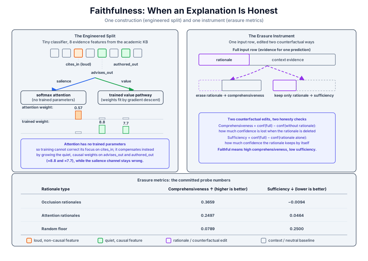One construction, one instrument: attention concentrates where gradients do not flow, and the erasure metrics catch it by the margins the committed table records. Original diagram by the authors, created with AI assistance.

The committed table, row by row

Three rationale extractors compete, each naming its top $k = 2$ features per probe example (faithfulness.py lines 346–354): attention takes the two highest attention weights, occlusion takes the two highest leave-one-out importances, and random draws two features uniformly. The ERASER instrument scores all three on the 512 held-out probe profiles:

[4] the ERASER instrument: both metrics, three extractors
    (comprehensiveness: higher = rationale was needed;
     sufficiency: lower = rationale alone already predicts)
    rationale (top-2)   comprehensiveness   sufficiency
    occlusion                      0.3659       -0.0094
    attention                      0.2497        0.0464
    random                         0.0789        0.2500

rationale	comprehensiveness (higher = needed)	sufficiency (lower = suffices)	what the numbers say
occlusion	$0.3659$	$-0.0094$	erasing it costs 37 points of confidence; alone, it predicts slightly better than the full input
attention	$0.2497$	$0.0464$	erasing it costs 25 points, but only because one causal feature leaks into the top-2
random	$0.0789$	$0.2500$	the floor: ignorance still scores, which is why the floor must be measured

Every number in the table decomposes into the importance column of the previous section, and working the decomposition is the best way to internalize what the metrics measure. The attention rationale is essentially always the pair (cites_in, advises_out): the saliences 2.5 and 1.2 dominate the $\pm 0.15$ jitter, so the loud spurious feature and exactly one causal feature fill the top-2. Erasing that pair deletes advises_out, whose single-feature importance is 0.2488, plus cites_in, worth 0.0004; the measured comprehensiveness 0.2497 is that sum, up to interaction. Its sufficiency, 0.0464, is the mirror image: keeping only that pair erases authored_out, whose importance is 0.0466. Attention's score is not zero, but it is propped up by the one causal feature that happens to be second-loudest; the metric correctly bills it for the causal feature it missed. The occlusion rationale names the causal pair exactly on 79.5% of examples, and its comprehensiveness 0.3659 exceeds the sum of the two single-feature importances ($0.2488 + 0.0466 = 0.2954$): both features push the same logit, and the sigmoid's nonlinearity makes the joint erasure cost more than its parts on this run. Its sufficiency is negative, $-0.0094$, meaning the causal pair alone predicts marginally better than the full input, since erasing the six noise features strips variance the model never wanted. The random floor is predictable from first principles: a uniform pair contains any given feature with probability $k/T = 2/8 = 0.25$, so its expected comprehensiveness is roughly $0.25 \times (0.2488 + 0.0466 + \dots) \approx 0.074$, and the committed 0.0789 sits just above that back-of-envelope value because of the same joint-erasure interaction on draws that hit both causal features. The chapter's claims are exactly the margins, and they are enforced as code (faithfulness.py lines 394–398):

    assert comp_occ >= comp_att + 0.05, "occlusion did not beat attention (comp)"
    assert comp_att >= comp_rnd + 0.05, "random was not worst on comprehensiveness"
    # Sufficiency (lower = better) runs the same way, by clear margins.
    assert suff_occ <= suff_att - 0.03, "occlusion did not beat attention (suff)"
    assert suff_rnd >= suff_att + 0.05, "random was not worst on sufficiency"

The real scholars, read through the model

The laboratory closes by reading the five actual knowledge-base people through the trained classifier, their feature profiles built by counting Volume 1's real edges and z-scoring per channel (faithfulness.py lines 293–325):

[5] the real kb scholars, read through the trained model
    person  advises_out  authored_out  cites_in  p(professor)  kb says
    alice             1             1         1        0.6370  professor
    bob               2             1         1        0.9132  professor
    carol             1             1         1        0.6319  student
    dave              0             1         0        0.2444  student
    erin              0             0         0        0.1166  student

The extremes come out right, and the harness asserts both: bob, who advises two people, is confidently a professor; erin, with no outgoing evidence at all, is confidently not (faithfulness.py lines 403–404). The instructive rows are alice and carol. The professor alice and the student carol (who already advises erin) present identical values on every channel the model relies on, and land within 0.0051 of each other, an agreement the harness asserts (faithfulness.py lines 405–406). No amount of faithfulness measurement can rescue a model whose evidence cannot distinguish two individuals; only Volume 2's typing axiom, Professor ⊓ Student ⊑ ⊥, tells alice and carol apart. Faithfulness is about whether the explanation reports the computation, not about whether the computation is adequate. Both questions matter, and only one of them is this chapter's.

The published record

The toy is engineered; the phenomenon is not. The record the chapter's instrument miniaturizes, cited for what each piece actually showed:

• Attention is substitutable. Across text-classification models with recurrent encoders, learned attention weights correlate weakly with gradient-based and leave-one-out feature importance, and one can find adversarial attention distributions, maximally different from the learned ones, that leave predictions essentially unchanged. The conclusion drawn was calibrated, not maximal: attention weights should not be treated as explanation by default [1].
• The counter-argument. Existence proofs of alternative attention are not counterfactuals about the trained model: the adversarial weights are imposed, not learned, and detached from the encoder that produced them. Under fair conditions (adversaries trained end to end, variance measured against random-seed baselines) attention is harder to replace than the adversarial construction suggests, and in some tasks it carries real signal. The debate's residue is methodological: whether attention explains is an empirical, per-model question requiring controlled tests [2].
• Standardization. ERASER turned the erasure idea into a benchmark: seven datasets with human rationale annotations, and comprehensiveness and sufficiency as the shared faithfulness metrics, computed exactly as defined above (with a variant that averages over rationale sizes). Its explicit distinction between agreement with human rationales (plausibility) and erasure behavior (faithfulness) is the same distinction this chapter opened with [3].
• The frontier version. For large language models explaining themselves in prose, the measured result is sobering: inject a biasing feature into a prompt (for example, reorder multiple-choice options so the correct answer is always at a fixed position, or plant a suggested answer), and models shift their answers while their chain-of-thought explanations systematically fail to mention the bias, instead constructing plausible support for the biased answer. The stated reasoning is demonstrably not the cause of the prediction, which is precisely comprehensiveness failing at the level of reasoning traces [4].

Trace-erasure: the volume's reusable instrument

Strip the laboratory away and one protocol remains, and it is the protocol this volume will keep reusing. Given a triple (model, input, explanation), the test is two-sided: erase the evidence the explanation cites, and the prediction must move; erase evidence the explanation does not cite, and the prediction must not. The companion's implementation is deliberately model-agnostic in shape, eraser_metrics(x, alpha, w, b, rationales) -> (comprehensiveness, sufficiency) (faithfulness.py lines 259–282): anything that can be predicted, and whose inputs can be selectively redacted, can be scored.

The protocol is already familiar in both directions along the series. Looking back, it is exactly how justifications were certified: minimality is trace-erasure with a reasoner as the model, where "the prediction must move" hardens into "the entailment must break", and the statistical metrics of this chapter are that theorem's degraded, measurable shadow. Looking forward, SATORI's claims table commits its faithfulness claim, C3, to exactly this measurement: the architecture's proof traces are to be scored by trace-erasure sufficiency and comprehensiveness against attention-rollout and gradient-saliency baselines, and the discretized trace must additionally re-verify as a genuine justification in Volume 2's sense (faithfulness.py lines 219–227 record the commitment beside the instrument). Part VII runs that evaluation. And the immediately next chapter needs the protocol's sibling: when the explanation is not a feature subset but an extracted rule set, the question becomes whether the rules agree with the model's predictions on unseen inputs, a metric called fidelity, which is trace-erasure lifted from evidence to behavior.

What the metrics cannot give

Passing the erasure test is necessary evidence of honesty; it is not a causal guarantee. The limits deserve the same precision as the definitions.

Erased inputs can be off-manifold. Occlusion evaluates the model on inputs unlike anything it was trained on: a profile with its features zeroed, a sentence with tokens deleted. The confidence drop then conflates two effects, the removal of information and the shock of an out-of-distribution input. The literature treats this as the erasure metrics' standing weakness: the ROAR protocol (RemOve And Retrain) retrains the model on erased inputs precisely to eliminate the confound [5], and ERASER's own aggregate variant notes that it reuses the trained model rather than retraining [3]. The companion sidesteps the confound by construction: erasure replaces a feature with its exact marginal mean, attention is held fixed (faithfulness.py lines 171–174), and the logit is linear in $x$ once attention is fixed, so there is no learned nonlinear response for an off-manifold input to shock. Real models get no such luxury.

Correlated features make "the" rationale non-unique. If two features carry the same signal, erasing either alone moves nothing (the other covers), and erasing both moves a lot; comprehensiveness of any single-feature rationale understates its causal role, and several different rationales pass the test equally well. The laboratory sidesteps this by generating independent features; the world does not. A passed test certifies a sufficient, needed rationale, not the unique one.

Faithfulness is relative to a granularity. This chapter measured explanations that cite input features. One can instead ask whether an explanation faithfully reports neurons, circuits, or algorithmic structure, and the conceptual map that disentangles these notions (plausibility, transparency at several grains, post-hoc explanation) makes clear they are different properties with different tests [6]. An explanation can be faithful at the feature level while misreporting the mechanism that combines the features.

None of this excuses skipping the test. It bounds what passing means: a model whose explanation fails erasure is telling a story that is measurably not the cause, and no appeal to correlation or granularity rescues it. The metrics are a filter that catches liars, not a certificate that crowns truth-tellers.

The unsolved part

The erasure protocol needs something to erase. A rationale that names features, tokens, retrieved documents, or proof steps has discrete, addressable parts, and the counterfactual is well defined: redact this part, re-run, compare. A free-form explanation has none of that. When a model explains itself in a paragraph of prose, the explanation's "parts" are claims, not tokens; deleting the sentence that states a reason does not delete the reason from the model's computation, and there is no agreed operation that does. The frontier measurements of chain-of-thought unfaithfulness [4] succeed by an end run: they perturb the input with a bias and check whether the explanation confesses, which detects dishonesty without ever scoring the explanation's content directly. A general faithfulness metric for free-form explanations, one that assigns a number to an arbitrary paragraph the way comprehensiveness assigns one to a feature subset, does not exist, and it is not obvious it can, since prose can always be paraphrased around any fixed erasure operator. The field's current best practice reads instead like an argument about architecture: if you want explanations you can audit, produce explanations with erasable structure, rationale spans, retrieved evidence, executable programs, proof traces. That is not a neutral observation in this series. It is a design pressure pointing directly at systems whose explanations are checkable by construction, which is where this volume is headed.

Why it matters

Volume 5 opened with the symbolic gold standard: a justification is minimal, verified, and faithful by theorem. This chapter is the first step down from that guarantee into the statistical world where the rest of the frontier lives, and the step is the volume's method in miniature: when a property cannot be proved, operationalize it, measure it against a floor, and assert the margins in committed code. The distinction between plausible and faithful will not stay confined to attention maps. It returns as fidelity in rule extraction, as the gap between confidence and correctness in the calibration chapter, as reasoning shortcuts in Part IV (models right for the wrong internal reasons, at scale), and as SATORI's C3 claim in Part VII, where the erasure instrument built here is aimed at proof traces. For the reader's own research the export is a habit: any time a system offers you its reasons, before admiring them, ask what happens when you take them away.

Key terms

• Plausible explanation: an explanation optimized for human acceptance; selective, fluent, judged by agreement with human priors or annotations, and logically independent of the model's computation.
• Faithful explanation: an explanation that accurately reports the causes of the model's output; judged by counterfactual tests on the model, not by appeal.
• Rationale: the explanation object under test here, a subset of input features (more generally: tokens, spans, evidence items) put forward as what the prediction rests on.
• Occlusion / erasure: replacing a feature's value with a neutral stand-in (here the population mean) to simulate its absence; itself a modeling choice whose artifacts the metrics inherit.
• Comprehensiveness: $p(\hat{y} \mid x) - p(\hat{y} \mid x \setminus r)$, the confidence lost when the rationale is erased; high means the rationale was needed.
• Sufficiency: $p(\hat{y} \mid x) - p(\hat{y} \mid r)$, the confidence lost when only the rationale remains; low (or negative) means the rationale alone carries the prediction.
• Random-rationale floor: the score of a uniformly random size-$k$ rationale; the calibration baseline both metrics require, and it is not zero.
• Occlusion importance: the single-feature version of comprehensiveness, the confidence drop when exactly one feature $x_t$ is erased; the attribution attention was compared against.
• Trace-erasure protocol: the general two-sided test: erase cited evidence, the prediction must move; erase uncited evidence, it must not. Justifications pass it by theorem; statistical explanations must pass it by measurement.
• Fidelity: the model-agreement analogue for extracted surrogate models: how often the extracted rules reproduce the model's predictions; next chapter's central metric.

Where this leads

Erasure scores an explanation that points at evidence. The next chapter raises the stakes on what an explanation can be: not a highlighted subset of the input but an entire symbolic surrogate, a set of rules extracted from the trained model that claims to reproduce its behavior. That claim has its own metric (fidelity: does the rule set agree with the model on inputs neither has seen?) and its own classic algorithms, from decision-tree queries in the style of TREPAN to the rule-from-weights tradition of KBANN (Knowledge-Based Artificial Neural Networks). Rule Extraction builds both, and inherits this chapter's discipline: a rule set that merely sounds like the model is plausibility; only measured agreement is faithfulness.

---

Companion code: examples/frontier/faithfulness.py implements the seeded laboratory, the frozen-attention classifier with its hand-derived gradient, occlusion importance, both ERASER metrics, the random floor, and the kb-scholar reading. Run python3 examples/frontier/faithfulness.py to reproduce every number in this chapter; the run is deterministic and every margin the chapter argues from is guarded by an assert.